Cocaine Dependence

Overview

In this vignette, we demonstrate the power of easyml using a Cocaine Dependence dataset.

Load the data

First we load our libraries and the Cocaine Dependence dataset.

library(easyml)

## Loaded easyml 0.1.1. Also loading ggplot2.

## Loading required namespace: ggplot2

library(dplyr)

## 
## Attaching package: 'dplyr'

## The following objects are masked from 'package:stats':
## 
##     filter, lag

## The following objects are masked from 'package:base':
## 
##     intersect, setdiff, setequal, union

library(ggplot2)

data("cocaine_dependence", package = "easyml")
knitr::kable(head(cocaine_dependence))

subject	age	male	edu_yrs	imt_comm_errors	imt_omis_errors	a_imt	b_d_imt	stop_ssrt	lnk_adjdd	lkhat_kirby	revlr_per_errors	bis_attention	bis_motor	bis_nonpl	igt_total
20031	29	0	16	6.90	5.51	0.97	-0.12	346.3	-5.848444	-5.227870	2	11	21	24	6
20044	33	0	17	15.63	13.27	0.92	-0.09	303.4	-9.026670	-5.832566	1	12	21	22	44
20053	57	0	13	25.44	16.41	0.87	-0.27	214.6	-6.115988	-4.014322	5	13	19	17	-16
20060	26	1	18	7.38	6.25	0.96	-0.09	190.2	-7.771655	-5.272179	3	14	21	17	52
20066	38	0	13	31.54	10.09	0.88	-0.61	273.9	-5.791562	-3.102204	5	11	20	23	-6
20081	41	0	17	43.33	33.87	0.69	-0.20	306.2	-3.766913	-3.676198	8	10	17	14	-22

Train a random forest model

To run an easy_random_forest model, we pass in the following parameters:

the data set cocaine_dependence,
the name of the dependent variable e.g. diagnosis,
whether to run a gaussian or a binomial model,
which variables to exclude from the analysis,
which variables are categorical variables; these variables are not scaled, if preprocess_scale is used,
the random state,
whether to display a progress bar,
how many cores to run the analysis on in parallel.

results <- easy_random_forest(cocaine_dependence, "diagnosis",
                              family = "binomial", 
                              exclude_variables = c("subject"),
                              categorical_variables = c("male"),
                              n_samples = 10, n_divisions = 10,
                              n_iterations = 2, progress_bar = FALSE, 
                              random_state = 12345, n_core = 1)

Assess results

Now let’s assess the results of the easy_random_forest model.

Estimates of variable importances

First, let’s examine the estimates of the variable importances.

results$plot_variable_importances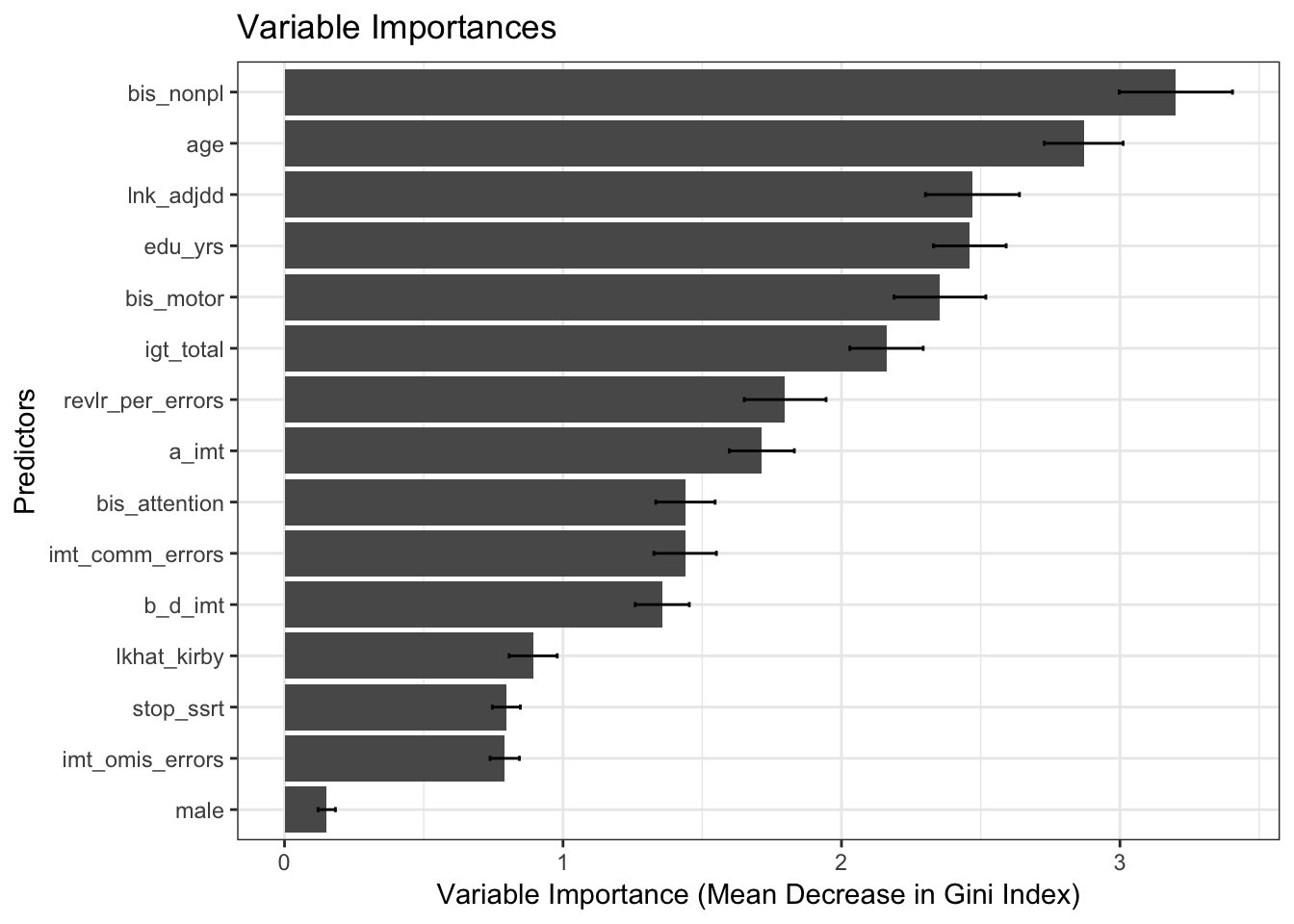

output <- results$variable_importances_processed
knitr::kable(output, digits  = 2)

predictor	mean	sd	lower_bound	upper_bound
age	2.87	0.14	2.73	3.01
male	0.15	0.03	0.12	0.18
edu_yrs	2.46	0.13	2.33	2.59
imt_comm_errors	1.44	0.11	1.33	1.55
imt_omis_errors	0.79	0.05	0.74	0.84
a_imt	1.71	0.12	1.60	1.83
b_d_imt	1.36	0.10	1.26	1.45
stop_ssrt	0.80	0.05	0.75	0.85
lnk_adjdd	2.47	0.17	2.30	2.64
lkhat_kirby	0.89	0.09	0.81	0.98
revlr_per_errors	1.80	0.15	1.65	1.94
bis_attention	1.44	0.11	1.33	1.55
bis_motor	2.35	0.16	2.19	2.52
bis_nonpl	3.20	0.20	3.00	3.40
igt_total	2.16	0.13	2.03	2.29

Predictions

We can examine both the in-sample and out-of-sample ROC curve plots for one particular trian-test split determined by the random state and determine the Area Under the Curve (AUC) as a goodness of fit metric. Here, we see that the in-sample AUC is higher than the out-of-sample AUC, but that both metrics indicate the model fits relatively well.

results$plot_predictions_single_train_test_split_train

## Warning: glm.fit: fitted probabilities numerically 0 or 1 occurred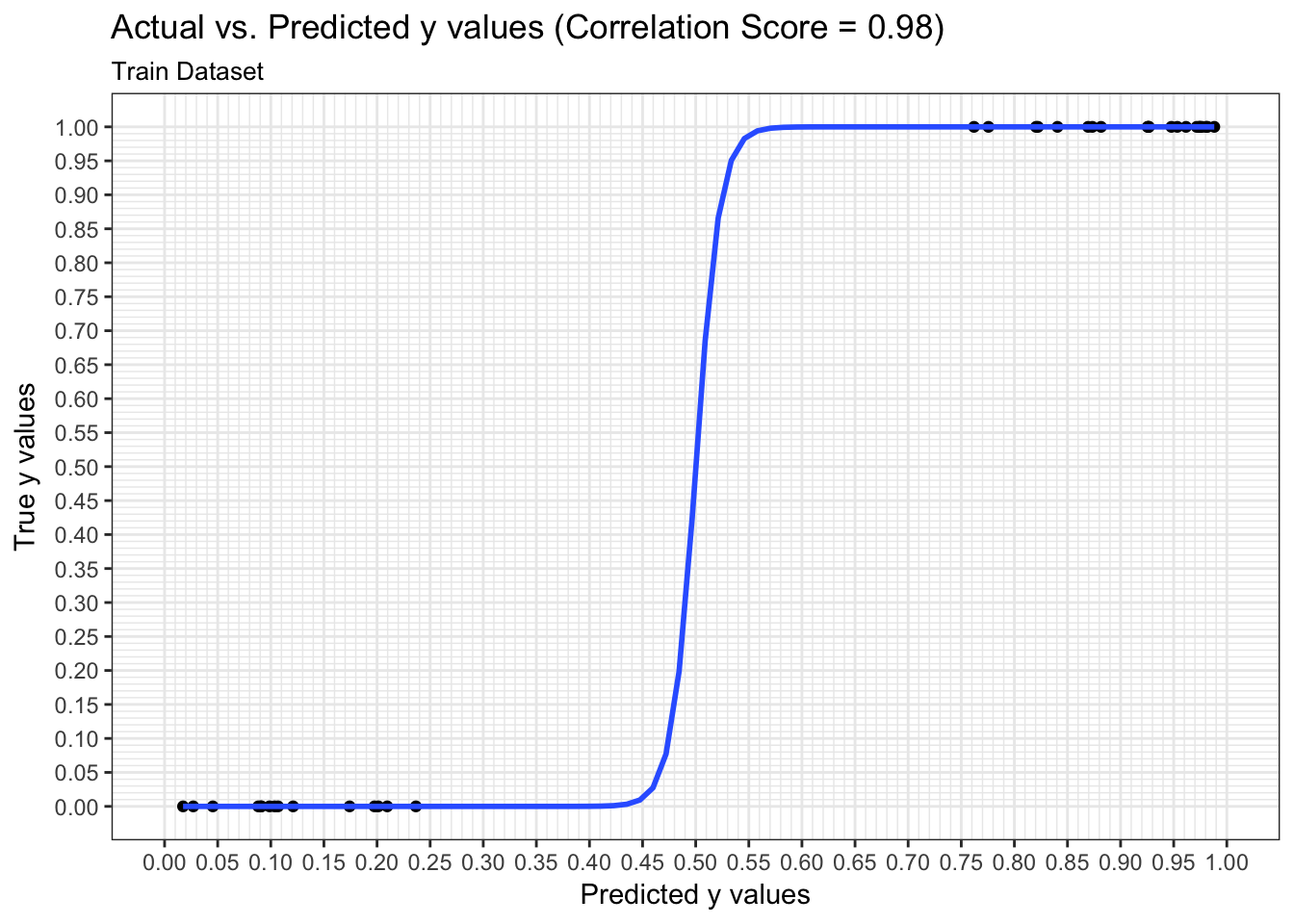

results$plot_predictions_single_train_test_split_test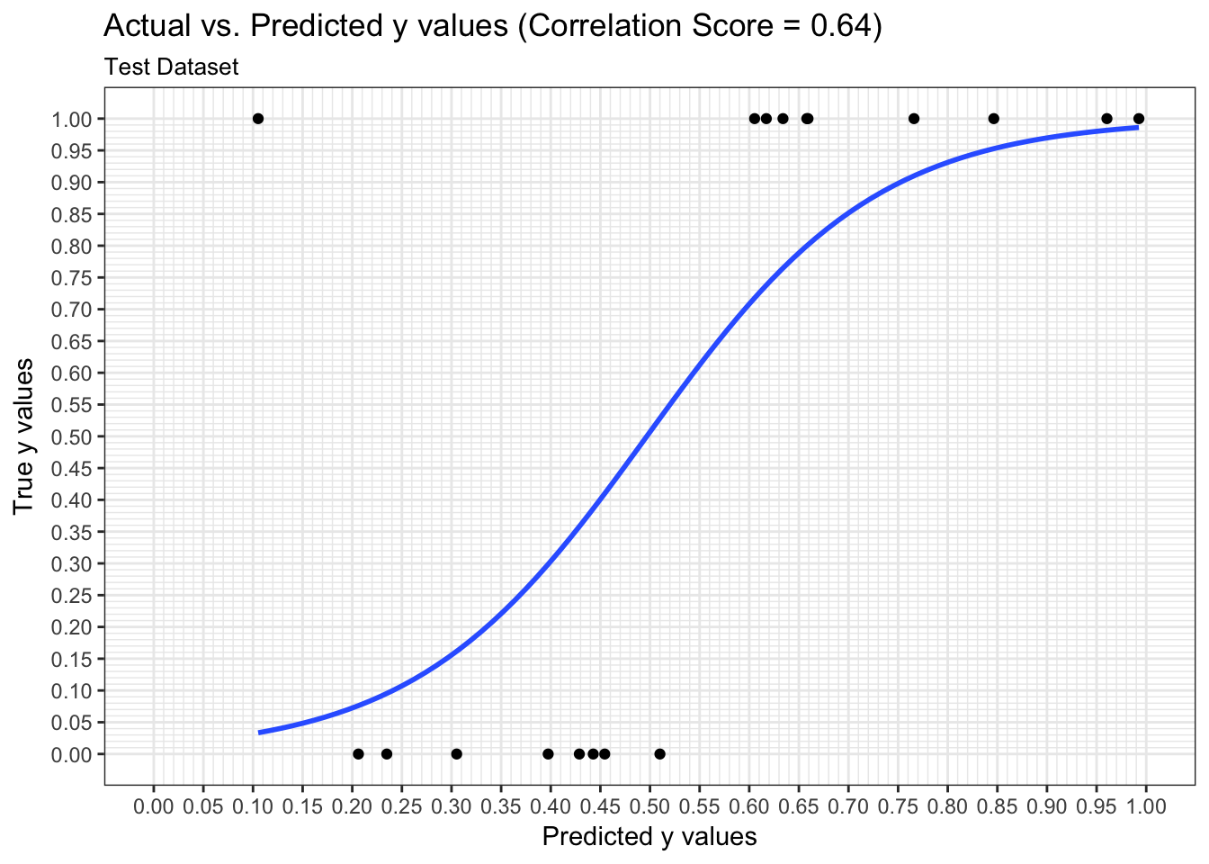

ROC Curve

We can examine both the in-sample and out-of-sample ROC curve plots for one particular trian-test split determined by the random state and determine the Area Under the Curve (AUC) as a goodness of fit metric. Here, we see that the in-sample AUC is higher than the out-of-sample AUC, but that both metrics indicate the model fits relatively well.

results$plot_roc_single_train_test_split_train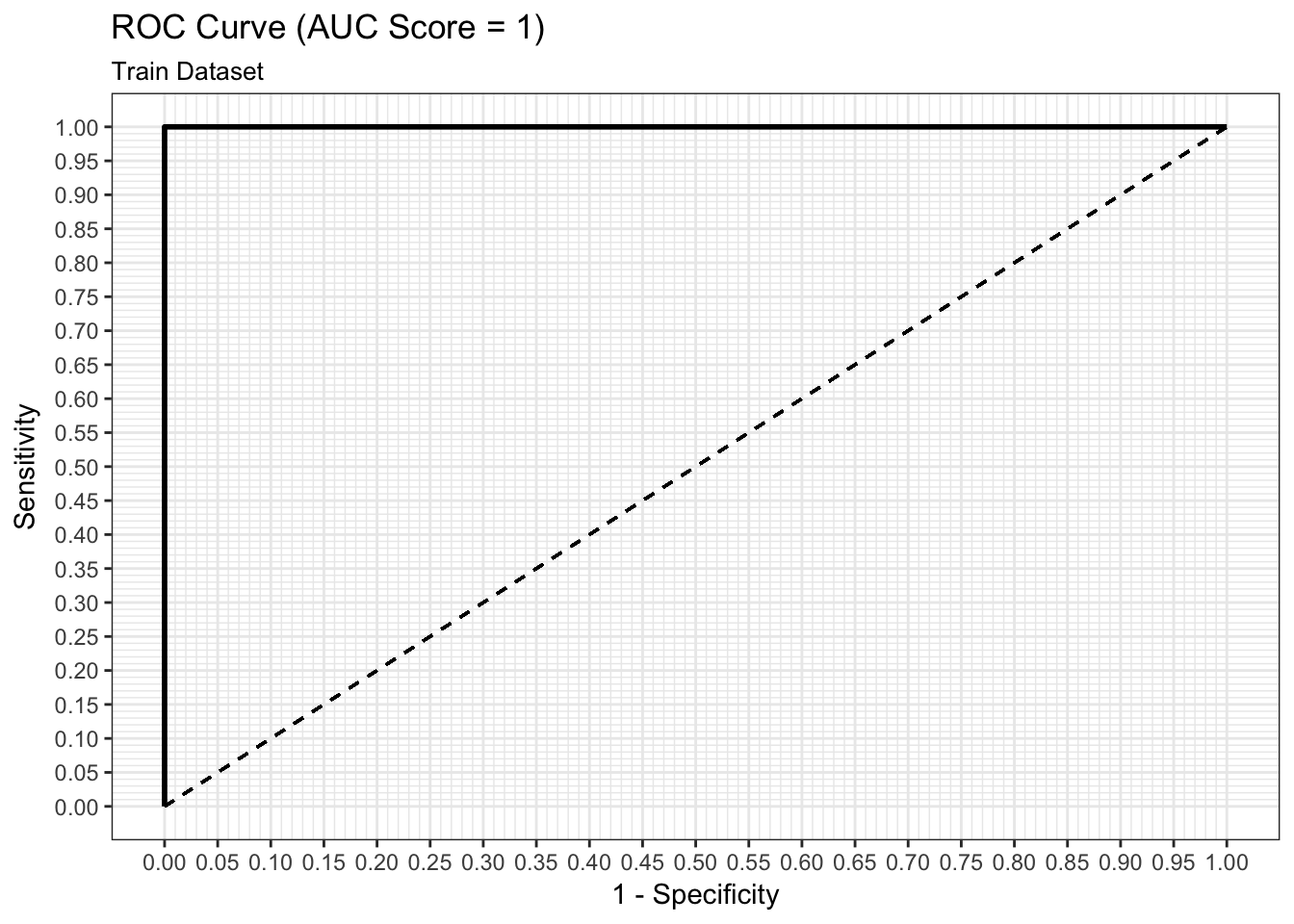

results$plot_roc_single_train_test_split_test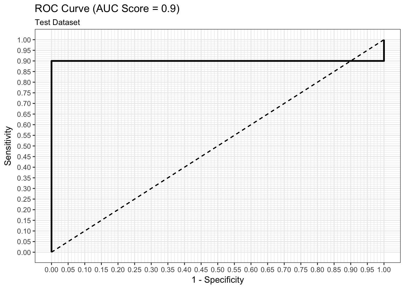

Model Performance

We can examine both the in-sample and out-of-sample AUC metrics for n_divisions train-test splits (ususally defaults to 1,000). Again, we see that the in-sample AUC is higher than the out-of-sample AUC, but that both metrics indicate the model fits relatively well.

results$plot_model_performance_train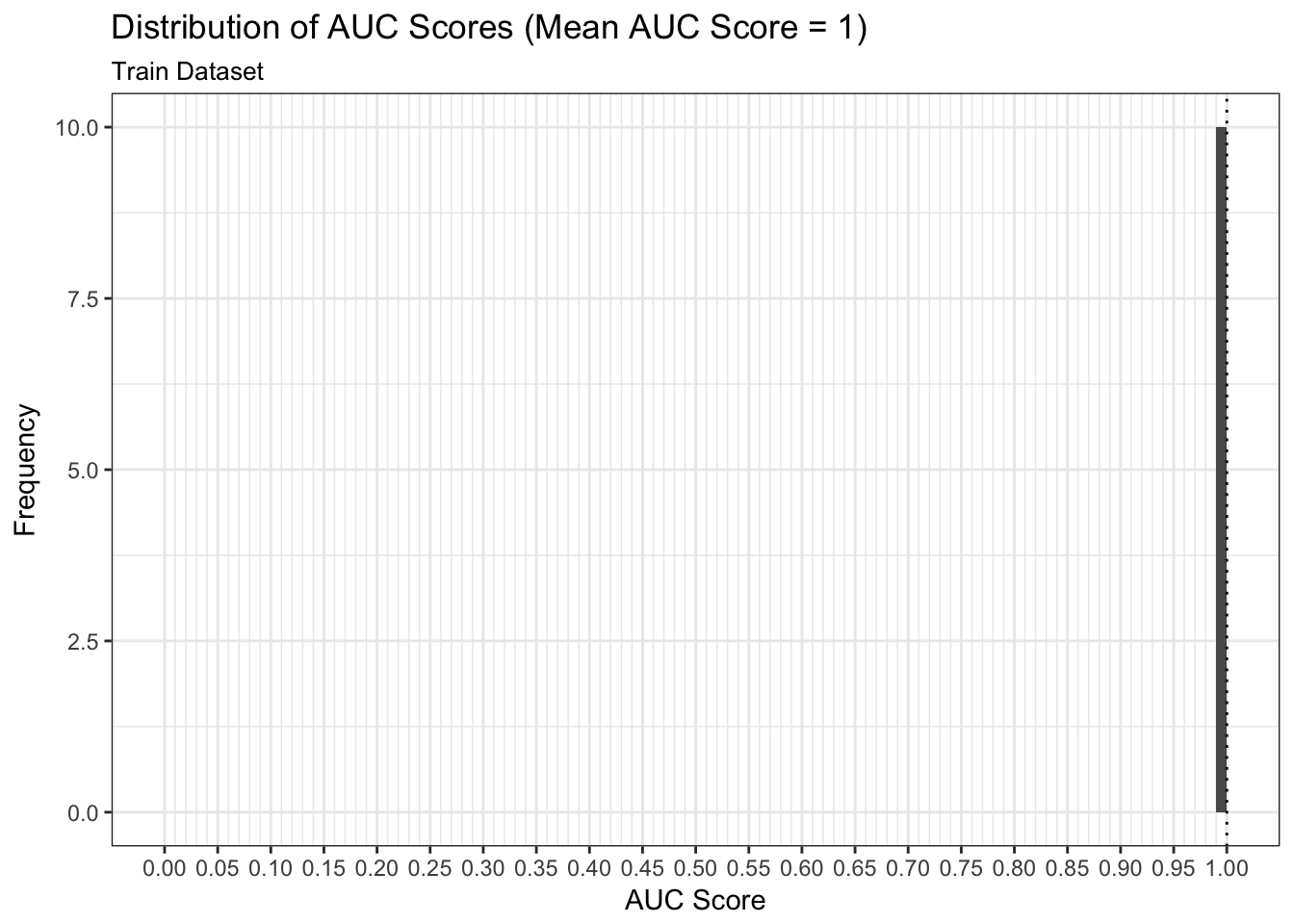

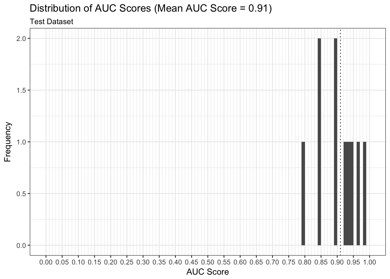
results$plot_model_performance_test

Discuss

In this vignette we used easyml to easily build and evaluate a random forest model using a Cocaine Dependence dataset.

Paul Hendricks

2017-07-08