Overview

In this vignette, we demonstrate the power of easyml using a Prostate Cancer dataset.

Load the data

First we load our libraries and the Prostate Cancer dataset.

library(easyml)

## Loaded easyml 0.1.1. Also loading ggplot2.

## Loading required namespace: ggplot2

library(dplyr)

## 
## Attaching package: 'dplyr'

## The following objects are masked from 'package:stats':
## 
##     filter, lag

## The following objects are masked from 'package:base':
## 
##     intersect, setdiff, setequal, union

library(ggplot2)

data("prostate", package = "easyml")
knitr::kable(head(prostate))

lcavol	lweight	age	lbph	svi	lcp	gleason	pgg45	lpsa
-0.5798185	2.769459	50	-1.386294	0	-1.386294	6	0	-0.4307829
-0.9942523	3.319626	58	-1.386294	0	-1.386294	6	0	-0.1625189
-0.5108256	2.691243	74	-1.386294	0	-1.386294	7	20	-0.1625189
-1.2039728	3.282789	58	-1.386294	0	-1.386294	6	0	-0.1625189
0.7514161	3.432373	62	-1.386294	0	-1.386294	6	0	0.3715636
-1.0498221	3.228826	50	-1.386294	0	-1.386294	6	0	0.7654678

Train a support vector machine model

To run an easy_support_vector_machine model, we pass in the following parameters:

• the data set prostate,
• the name of the dependent variable e.g. lpsa,
• whether to run a gaussian or a binomial model,
• how to preprocess the data; in this case, we use preprocess_scale to scale the data,
• the random state,
• whether to display a progress bar,
• how many cores to run the analysis on in parallel.

results <- easy_support_vector_machine(prostate, "lpsa", 
                                       n_samples = 10, n_divisions = 10, 
                                       n_iterations = 2, random_state = 12345, 
                                       n_core = 1)

## [1] "Generating predictions for a single train test split:"
## [1] "Generating measures of model performance over multiple train test splits:"

Assess results

Now let’s assess the results of the easy_support_vector_machine model.

Predictions: ROC Curve

We can examine both the in-sample and out-of-sample ROC curve plots for one particular trian-test split determined by the random state and determine the Area Under the Curve (AUC) as a goodness of fit metric. Here, we see that the in-sample AUC is higher than the out-of-sample AUC, but that both metrics indicate the model fits relatively well.

results$plot_predictions_single_train_test_split_train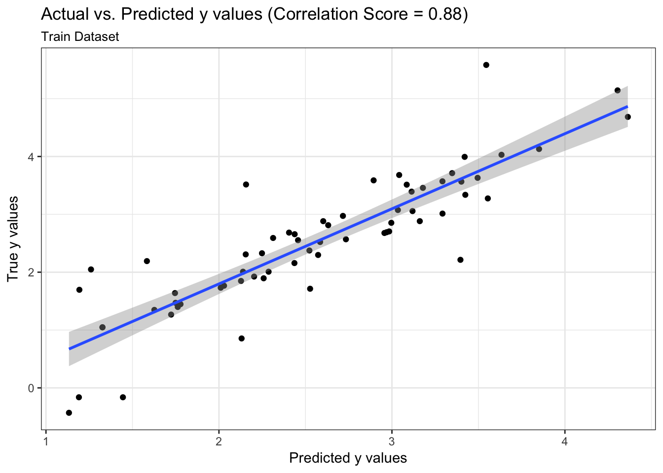

results$plot_predictions_single_train_test_split_test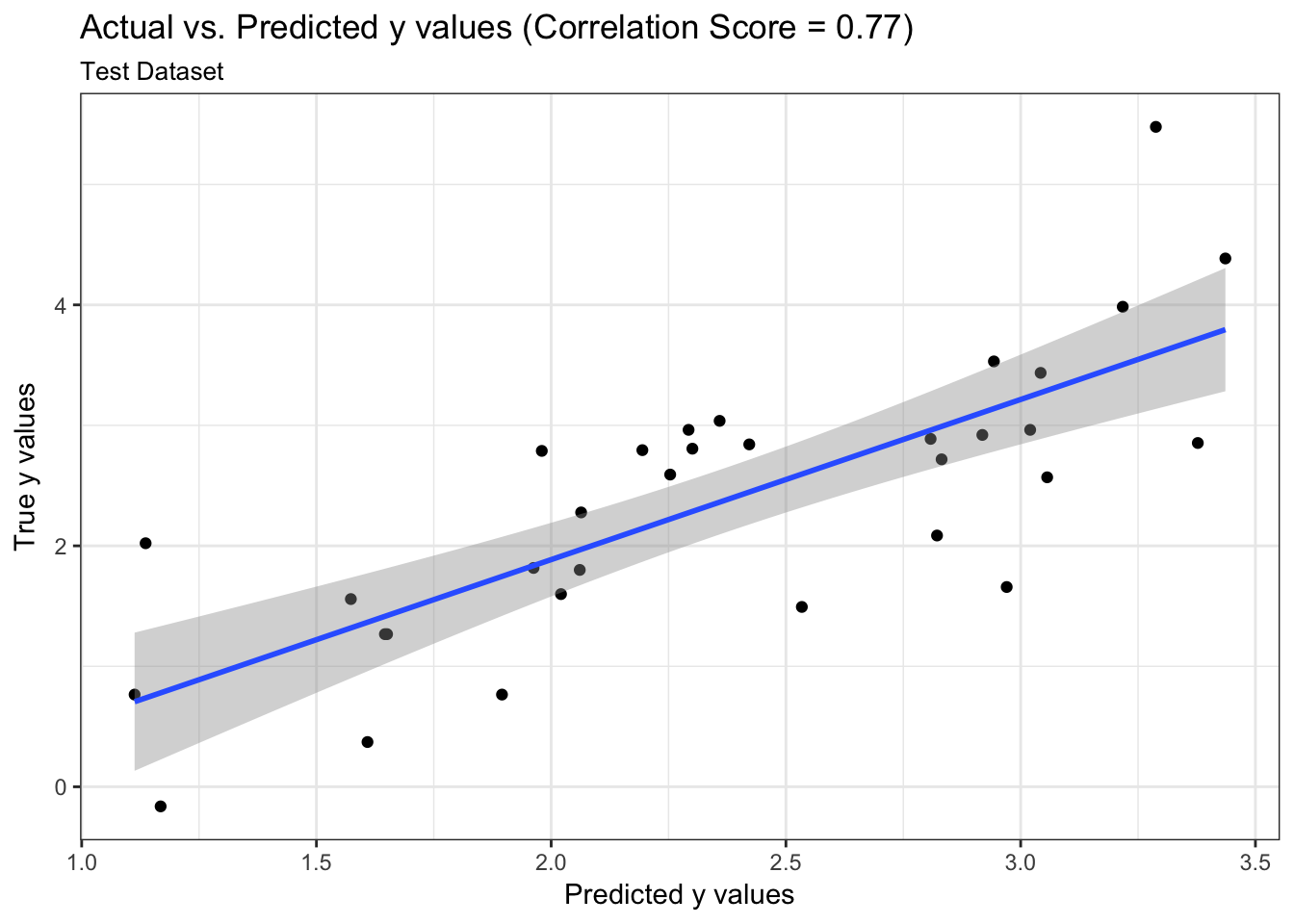

Metrics: AUC

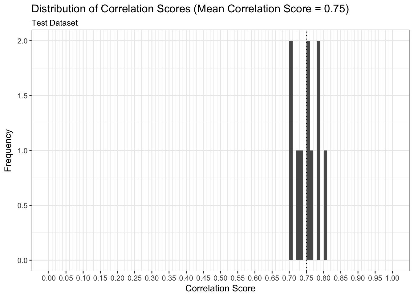
We can examine both the in-sample and out-of-sample AUC metrics for n_divisions train-test splits (ususally defaults to 1,000). Again, we see that the in-sample AUC is higher than the out-of-sample AUC, but that both metrics indicate the model fits relatively well.

results$plot_model_performance_train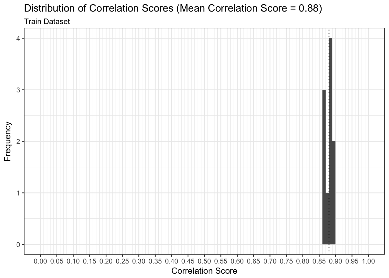

results$plot_model_performance_test

Discuss

In this vignette we used easyml to easily build and evaluate a support vector machine model using a Prostate Cancer dataset.