Surviving the Titanic
Paul Hendricks
2017-07-08
Load the data
Install the titanic package from CRAN. This package contains datasets providing information on the fate of passengers on the fatal maiden voyage of the ocean liner “Titanic”, with variables such as economic status (class), sex, age and survival. These data sets are often used as an introduction to machine learning on Kaggle. More details about the dataset can be found there.
library(easyml)## Loaded easyml 0.1.1. Also loading ggplot2.## Loading required namespace: ggplot2library(titanic)
library(dplyr)##
## Attaching package: 'dplyr'## The following objects are masked from 'package:stats':
##
## filter, lag## The following objects are masked from 'package:base':
##
## intersect, setdiff, setequal, unionlibrary(ggplot2)
data("titanic_train", package = "titanic")
knitr::kable(head(titanic_train))| PassengerId | Survived | Pclass | Name | Sex | Age | SibSp | Parch | Ticket | Fare | Cabin | Embarked |
|---|---|---|---|---|---|---|---|---|---|---|---|
| 1 | 0 | 3 | Braund, Mr. Owen Harris | male | 22 | 1 | 0 | A/5 21171 | 7.2500 | S | |
| 2 | 1 | 1 | Cumings, Mrs. John Bradley (Florence Briggs Thayer) | female | 38 | 1 | 0 | PC 17599 | 71.2833 | C85 | C |
| 3 | 1 | 3 | Heikkinen, Miss. Laina | female | 26 | 0 | 0 | STON/O2. 3101282 | 7.9250 | S | |
| 4 | 1 | 1 | Futrelle, Mrs. Jacques Heath (Lily May Peel) | female | 35 | 1 | 0 | 113803 | 53.1000 | C123 | S |
| 5 | 0 | 3 | Allen, Mr. William Henry | male | 35 | 0 | 0 | 373450 | 8.0500 | S | |
| 6 | 0 | 3 | Moran, Mr. James | male | NA | 0 | 0 | 330877 | 8.4583 | Q |
Tidy the data
To prepare the data for modeling, we will undergo the following steps:
- Filter out any places where
EmbarkedisNA, - Add together
SibSp,Parch, and1Lto estimate family size, - Create binary variables for each of the 2nd and 3rd class memberships,
- Create a binary for gender,
- Create binary variables for 2 of the ports of embarkation,
- Impute mean values of age where
AgeisNA.
titanic_train_2 <- titanic_train %>%
  filter(!is.na(Embarked), Embarked != "") %>%
  mutate(Family_Size = SibSp + Parch + 1L) %>%
  mutate(Pclass = as.character(Pclass)) %>%
  mutate(Pclass_3 = 1 * (Pclass == "3")) %>%
  mutate(Sex = 1 * (Sex == "male")) %>%
  mutate(Embarked_Q = 1 * (Embarked == "Q")) %>%
  mutate(Embarked_S = 1 * (Embarked == "S")) %>%
  mutate(Age = ifelse(is.na(Age), mean(Age, na.rm = TRUE), Age))
Train a penalized logistic model
To run an easy_glmnet model, we pass in the following parameters:
- the data set
titanic_train_2, - the name of the dependent variable e.g.
Survived, - whether to run a
gaussianor abinomialmodel, - how to preprocess the data; in this case, we use
preprocess_scaleto scale the data, - which variables to exclude from the analysis,
- which variables are categorical variables; these variables are not scaled, if
preprocess_scaleis used, - the random state,
- whether to display a progress bar,
- how many cores to run the analysis on in parallel.
.exclude_variables <- c("PassengerId", "Pclass", "Name",
                        "Ticket", "Cabin", "Embarked")
.categorical_variables <- c("Sex", "SibSp", "Parch", "Family_Size",
                            "Pclass_3", "Embarked_Q", "Embarked_S")
results <- easy_glmnet(titanic_train_2, "Survived",
                       family = "binomial",
                       preprocess = preprocess_scale,
                       exclude_variables = .exclude_variables,
                       categorical_variables = .categorical_variables,
                       random_state = 12345, progress_bar = FALSE,
                       n_samples = 10, n_divisions = 10,
                       n_iterations = 2, n_core = 1)
Assess results
Now let’s assess the results of the easy_glmnet model.
Estimates of weights
We can interpret the weights in the following way:
- A 1 standard deviation increase in
Fareincreases the log-odds of survival by 0.25 units, - For every unit increase in a passenger’s family size, the log-odds of survival decrease by 0.09 units,
- For every additional Sibling or Spouse in a passenger’s family, the log-odds of survival decrease by 0.17 units,
- A 1 standard deviation increase in
Agedecreases the log-odds of survival by 0.37 units, - If a passenger embarked at the Southampton port, the log-odds of survival decrease by 0.47 units,
- If a passenger is third class, the log-odds of survival decrease by 1.44 units,
- If a passenger is male, the log-odds of survival decrease by 2.53 units.
results$plot_coefficients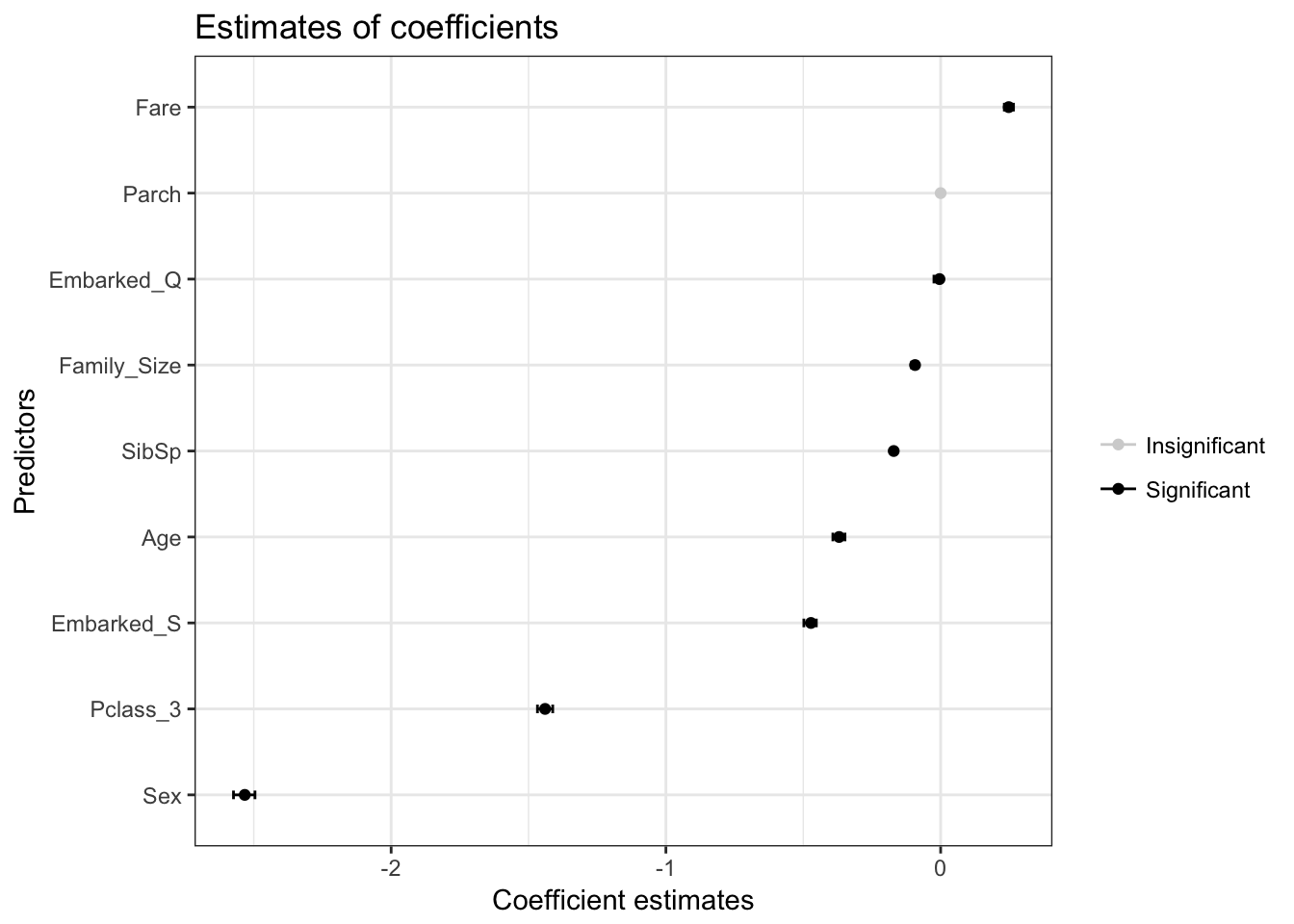
| predictor | mean | sd | lower_bound | upper_bound | survival | sig | dot_color_1 | dot_color_2 | dot_color |
|---|---|---|---|---|---|---|---|---|---|
| Fare | 0.25 | 0.01 | 0.23 | 0.27 | 1 | 1 | 1 | 2 | 2 |
| Parch | 0.00 | 0.00 | 0.00 | 0.00 | 0 | 0 | 0 | 1 | 0 |
| Embarked_Q | 0.00 | 0.01 | -0.02 | 0.00 | 1 | 1 | 1 | 2 | 2 |
| Family_Size | -0.09 | 0.01 | -0.11 | -0.08 | 1 | 1 | 1 | 2 | 2 |
| SibSp | -0.17 | 0.01 | -0.18 | -0.16 | 1 | 1 | 1 | 2 | 2 |
| Age | -0.37 | 0.01 | -0.39 | -0.35 | 1 | 1 | 1 | 2 | 2 |
| Embarked_S | -0.47 | 0.01 | -0.50 | -0.45 | 1 | 1 | 1 | 2 | 2 |
| Pclass_3 | -1.44 | 0.02 | -1.47 | -1.41 | 1 | 1 | 1 | 2 | 2 |
| Sex | -2.53 | 0.03 | -2.57 | -2.50 | 1 | 1 | 1 | 2 | 2 |
Predictions: ROC Curve
We can examine both the in-sample and out-of-sample ROC curve plots for one particular trian-test split determined by the random state and determine the Area Under the Curve (AUC) as a goodness of fit metric. Here, we see that the in-sample AUC is higher than the out-of-sample AUC, but that both metrics indicate the model fits relatively well.
results$plot_predictions_single_train_test_split_train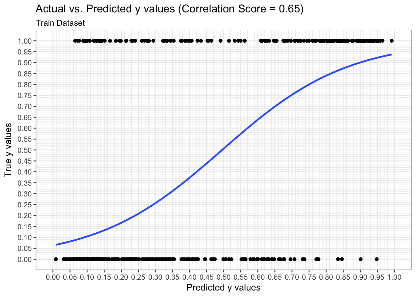
results$plot_predictions_single_train_test_split_test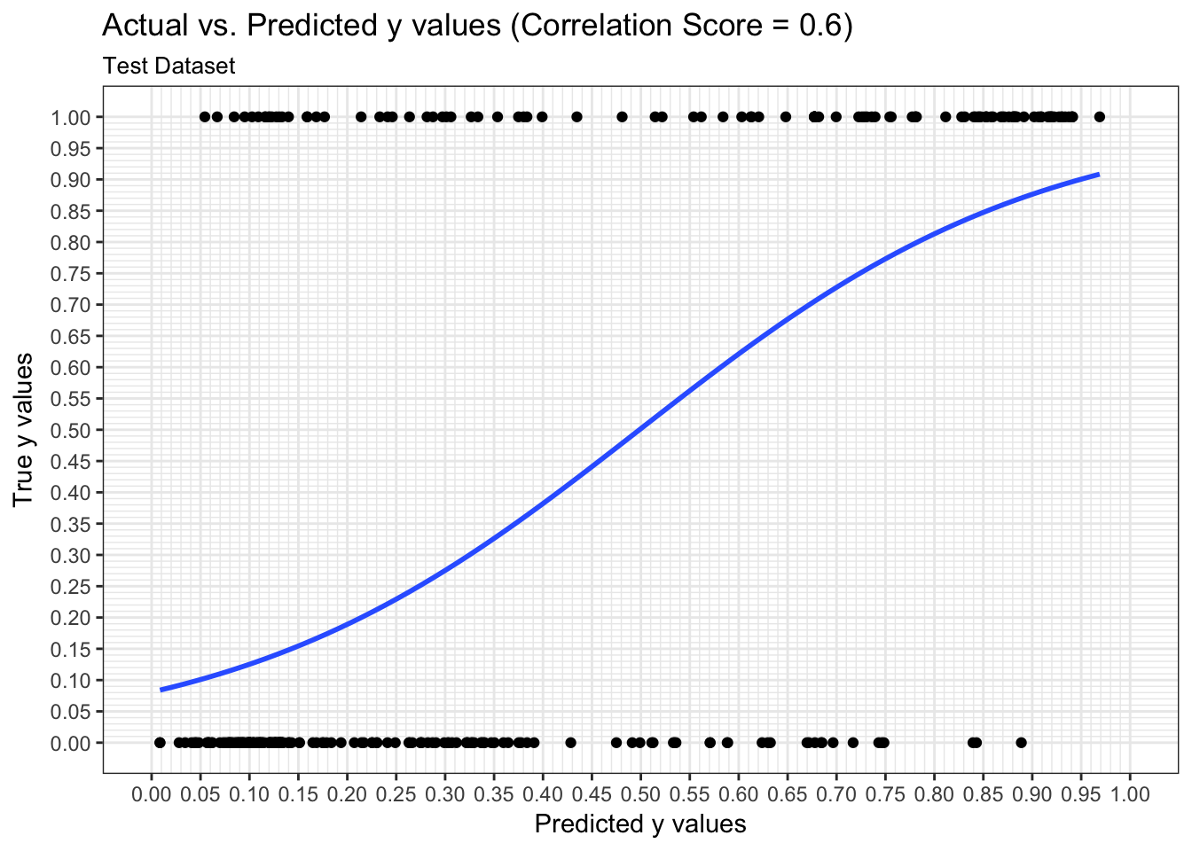
Metrics: AUC
We can examine both the in-sample and out-of-sample AUC metrics for n_divisions train-test splits (ususally defaults to 1,000). Again, we see that the in-sample AUC is higher than the out-of-sample AUC, but that both metrics indicate the model fits relatively well.
results$plot_model_performance_train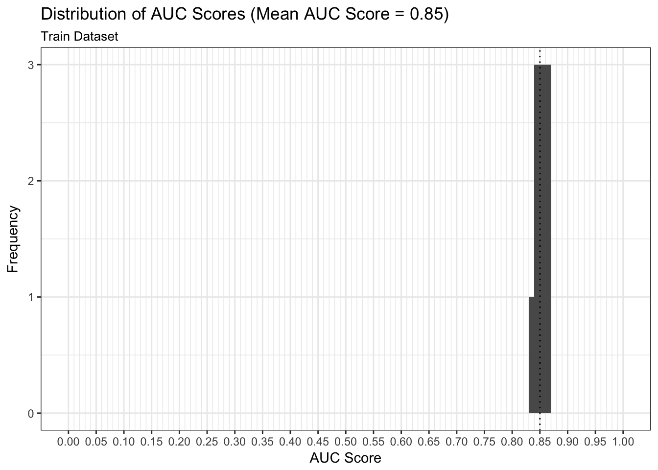
results$plot_model_performance_test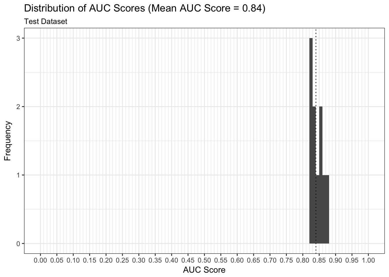
Discuss
In this vignette we used easyml to easily build and evaluate a penalized binomial regression model to assess the likelihood of passenger surival given a number of attributes. We can continue to finetune the model and identify the most optimal alpha/lambda hyperparameter combination; however, our estimates of the weights make intutive sense and a mean out-of-sample AUC of 0.85 right off the bat is indicative of a good model.