Getting Started

hBayesDM (hierarchical Bayesian modeling of Decision-Making tasks) is a user-friendly R package that offers hierarchical Bayesian analysis of various computational models on an array of decision-making tasks. Click here to download its help file (reference manual). Click here to read our paper published in Computational Psychiatry. Click here to download a poster we presented at several conferences/meetings. You can find hBayesDM on CRAN and GitHub.

Motivation

Computational modeling provides a quantitative framework for investigating latent neurocognitive processes (e.g., learning rate, reward sensitivity) and interactions among multiple decision-making systems. Parameters of a computational model reflect psychologically meaningful individual differences: thus, getting accurate parameter estimates of a computational model is critical to improving the interpretation of its findings. Hierarchical Bayesian analysis (HBA) is regarded as the gold standard for parameter estimation, especially when the amount of information from each participant is small (see below “Why hierarchical Bayesian analysis?”). However, many researchers interested in HBA often find the approach too technical and challenging to be implemented.

We introduce a free R package hBayesDM, which offers HBA of various computational models on an array of decision-making tasks (see below for a list of tasks and models currently available). Users can perform HBA of various computational models with a single line of coding. Example datasets are also available. With hBayesDM, we hope anyone with minimal knowledge of programming can take advantage of advanced computational modeling and HBA. It is our expectation that hBayesDM will contribute to the dissemination of these computational tools and enable researchers in related fields to easily characterize latent neurocognitive processes within their study populations.

Why hierarchical Bayesian analysis (HBA)?

Most computational models do not have closed form solutions and we need to estimate parameter values. Traditionally parameters are estimated at the individual level with maximum likelihood estimation (MLE): getting point estimates for each individual separately. However, individual MLE estimates are often noisy especially when there is insufficient amount of data. A group-level analysis (e.g., group-level MLE), which estimate a single set of parameters for the whole group of individuals, may generate more reliable estimates but inevitably ignores individual differences.

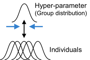
HBA and other hierarchical approaches (e.g., Huys et al., 2011) allow for individual differences while pooling information across individuals. Both individual and group parameter estimates (i.e., posterior distributions) are estimated simultaneously in a mutually constraining fashion. Consequently, individual parameter estimates tend to be more stable and reliable because commonalities among individuals are captured and informed by the group tendencies (e.g., Ahn et al., 2011). HBA also finds full posterior distributions instead of point estimates (thus providing rich information about the parameters). HBA also makes it easy to do group comparisons in a Bayesian fashion (e.g., comparing clinical and non-clinical groups, see an example below).

HBA is a branch of Bayesian statistics and the conceptual framework of Bayesian data analysis is clearly written in Chapter 2 of John Kruschke’s book (Kruschke, 2014). In Bayesian statistics, we assume prior beliefs (i.e., prior distributions) for model parameters and update the priors into posterior distributions given the data (e.g., trial-by-trial choices and outcomes) using Bayes’ rule. Note that the prior distributions we use for model parameters are vague (e.g., flat) or weakly informative priors, so they play a minimal role in the posterior distribution.

For Bayesian updating, we use the Stan software package (https://mc-stan.org/), which implements a very efficient Markov Chain Monte Carlo (MCMC) algorithm called Hamiltonian Monte Carlo (HMC). HMC is known to be effective and works well even for large complex models. See Stan reference manual (https://mc-stan.org/documentation/) and Chapter 14 of Kruschke (2014) for a comprehensive description of HMC and Stan. What is MCMC and why should we use it? Remember, we need to update our priors into posterior distributions in order to make inference about model parameters. Simply put, MCMC is a way of approximating a posterior distribution by drawing a large number of samples from it. MCMC algorithms are used when posterior distributions cannot be analytically achieved or using MCMC is more efficient than searching for the whole grid of parameter space (i.e., grid search). To learn more about the basic foundations of MCMC, we recommend Chapter 7 of Kruschke (2014).

Users can read our Stan source files to see how each model is implemented (e.g., pathTo_gng_m1 = system.file("stan_files/gng_m1.stan", package="hBayesDM")). We made strong efforts to optimize Stan codes through reparameterization (e.g., Matt trick) and vectorization.

Prerequisites

R ≥ 4.4 (cran.r-project.org).
CmdStan, installed via cmdstanr. hBayesDM uses cmdstanr (not rstan) to compile and run Stan models. CmdStan ships as a system dependency rather than a CRAN package — install it once with cmdstanr::install_cmdstan().
RStudio is optional but recommended.

Additional CRAN packages (ggplot2, loo, bayesplot, posterior, …) install automatically with hBayesDM.

Tasks & models implemented in hBayesDM

See here for the list of tasks and models implemented in hBayesDM.

How to install hBayesDM

1. Install cmdstanr and CmdStan

cmdstanr is hosted on the Stan r-universe rather than CRAN:

install.packages(
  "cmdstanr",
  repos = c("https://stan-dev.r-universe.dev", getOption("repos"))
)

# One-time CmdStan toolchain install (~5 min)
cmdstanr::install_cmdstan()

Verify the toolchain works by fitting any Stan model — for example, cmdstanr::cmdstanr_example("schools") runs a small “Eight Schools” fit without hBayesDM.

2. Install hBayesDM

From CRAN:

install.packages("hBayesDM")

From GitHub:

if (!require(remotes)) install.packages("remotes")
remotes::install_github("CCS-Lab/hBayesDM", subdir = "R")

First-fit compile cost

Stan models compile on first use (~30 s per model) and cmdstanr caches the compiled binary alongside the .stan file. Subsequent fits of the same model reuse the cached binary and start sampling immediately.

How to use hBayesDM

First, open RStudio (or just R) and load the package:

library(hBayesDM)

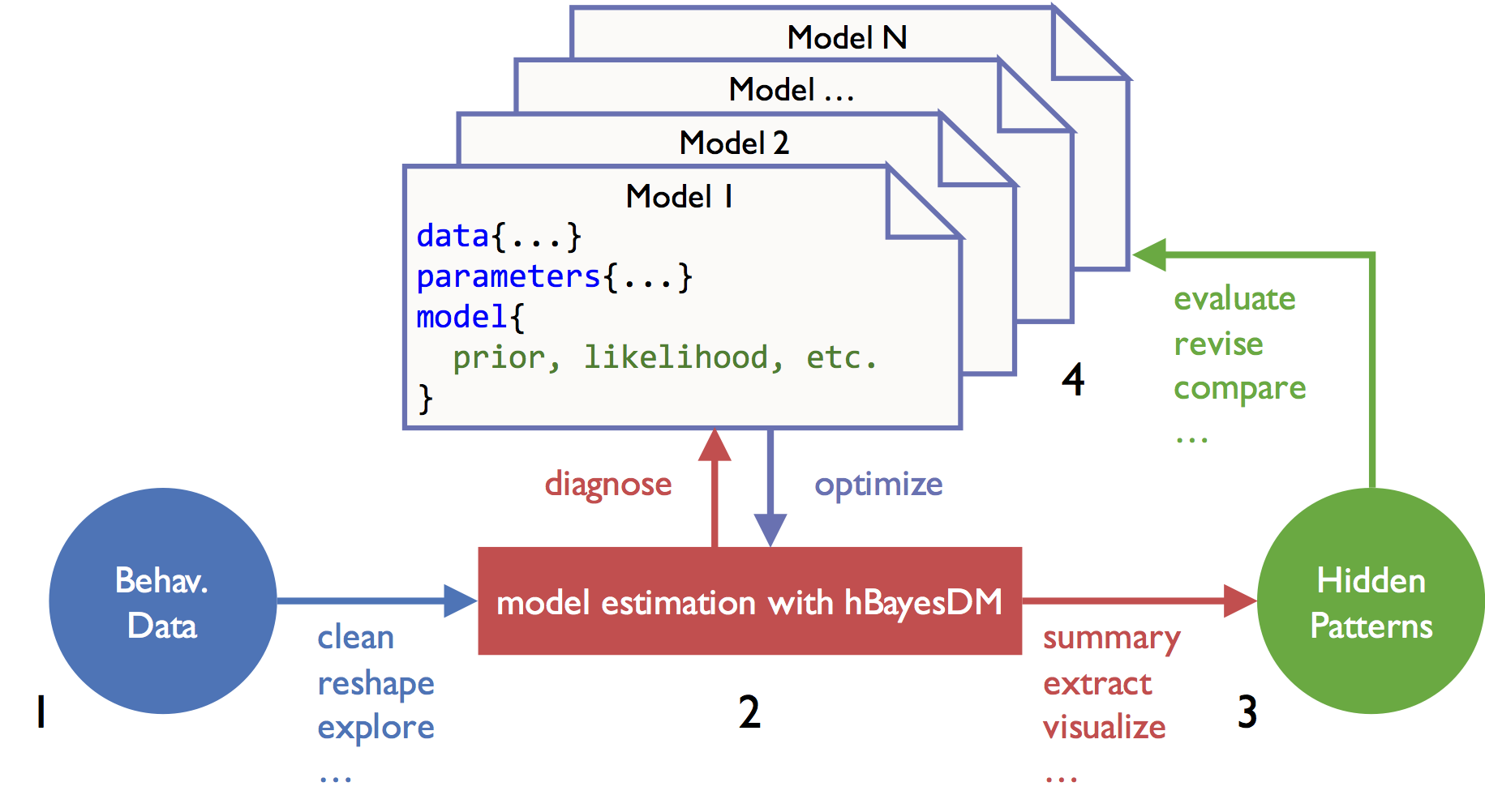
Four steps of doing HBA with hBayesDM are illustrated below. As an example, four models of the orthogonalized Go/Nogo task (Guitart-Masip et al., 2012; Cavanagh et al., 2013) are fit and compared with the hBayesDM package.

1) Prepare the data

For fitting a model with hBayesDM, all subjects’ data should be combined into a single text file (*.txt). Look at the sample dataset and a help file (e.g., ?gng_m1) for each task and carefully follow the instructions.
Subjects’ data must contain variables that are consistent with the column names specified in the help file, though extra variables are in practice allowed.
It is okay if the number of trials is different across subjects. But there should exist no N/A data. If some trials contain N/A data (e.g., choice=NA in trial#10), remove the trials first.
Sample data are available here, although users can fit a model with sample data without separately downloading them with one of the function arguments. Once the hBayesDM package is installed, sample data can be also retrieved from the package folder. Note that the file name of sample (example) data for a given task is taskName_exampleData.txt (e.g., dd_exampleData.txt, igt_exampleData.txt, gng_exampleData.txt, etc.). See each model’s help file (e.g., ?gng_m1) to check required data columns and their labels.

dataPath = system.file("extdata/gng_exampleData.txt", package="hBayesDM")

If you download the sample data to “~/Downloads”, you may specify the path to the data file like this:

dataPath = "~/Downloads/gng_exampleData.txt"

2) Fit candidate models

Below the gng_m1 model is fit on its example data. The command runs four MCMC chains across four cores. If you pass "example" as data, hBayesDM loads the bundled example file for that task. You can also assign your own initial values via the inits argument (e.g., inits = c(0.1, 0.2, 1.0)).

output1 = gng_m1(data="example", niter=2000, nwarmup=1000, nchain=4, ncore=4)

Equivalent shorter form (the defaults are 2000 / 1000 / 4 chains for gng models):

output1 = gng_m1("example", ncore=4)

## Warning in gng_m1(data = "example", niter = 2000, nwarmup = 1000, nchain = 4, : Number of cores specified for parallel computing greater than number of locally available cores. Using all locally available cores.

## 
## Model name  = gng_m1 
## Data file   = example 
## 
## Details:
##  # of chains                    = 4 
##  # of cores used                = 3 
##  # of MCMC samples (per chain)  = 2000 
##  # of burn-in samples           = 1000 
##  # of subjects                  = 10 
##  # of (max) trials per subject  = 240 
## 
## 
## ****************************************
## ** Use VB estimates as initial values **
## ****************************************
## ------------------------------------------------------------ 
## EXPERIMENTAL ALGORITHM: 
##   This procedure has not been thoroughly tested and may be unstable 
##   or buggy. The interface is subject to change. 
## ------------------------------------------------------------ 
## Gradient evaluation took 0.000601 seconds 
## 1000 transitions using 10 leapfrog steps per transition would take 6.01 seconds. 
## Adjust your expectations accordingly! 
## Begin eta adaptation. 
## Iteration:   1 / 250 [  0%]  (Adaptation) 
## Iteration:  50 / 250 [ 20%]  (Adaptation) 
## Iteration: 100 / 250 [ 40%]  (Adaptation) 
## Iteration: 150 / 250 [ 60%]  (Adaptation) 
## Iteration: 200 / 250 [ 80%]  (Adaptation) 
## Success! Found best value [eta = 1] earlier than expected. 
## Begin stochastic gradient ascent. 
##   iter             ELBO   delta_ELBO_mean   delta_ELBO_med   notes  
##    100         -846.796             1.000            1.000 
##    200         -815.045             0.519            1.000 
##    300         -809.962             0.348            0.039 
##    400         -809.490             0.261            0.039 
##    500         -810.612             0.209            0.006   MEDIAN ELBO CONVERGED 
## Drawing a sample of size 1000 from the approximate posterior...  
## COMPLETED. 
## Finished in  3.4 seconds.
## 
## ************************************
## **** Model fitting is complete! ****
## ************************************

On first use cmdstanr compiles the Stan model (~30 s); subsequent fits of the same model reuse the cached binary. Sampling for gng_m1 on the example data then takes 2–3 minutes. Occasional “numerical problems” warnings during warmup or a small number of “divergent transitions after warmup” can usually be ignored — see Stan’s Runtime warnings and convergence problems for guidance on when to act on them.

The hBayesDM console output looks like:

Model  = gng_m1
Data   = example

Details:
 # of chains                    = 4
 # of cores used                = 4
 # of MCMC samples (per chain)  = 2000
 # of burn-in samples           = 1000
 # of subjects                  = 10
 # of (max) trials per subject  = 240

Running MCMC with 4 parallel chains...

Chain 1 Iteration:    1 / 2000 [  0%]  (Warmup)
Chain 2 Iteration:    1 / 2000 [  0%]  (Warmup)
...

When fitting is complete:

************************************
**** Model fitting is complete! ****
************************************

output1 is an object of class hBayesDM with these fields:

model: Name of the fitted model (output1$model is "gng_m1").
all_ind_pars: Per-subject parameter summaries (default: mean). Use ind_pars = "median" or ind_pars = "mode" to change the summary statistic.
par_vals: Posterior draws as a named list, extracted via posterior::draws_of(). Hyper-parameters are prefixed mu_ (e.g., mu_xi, mu_ep, mu_rho).
fit: A CmdStanMCMC object (or CmdStanVB when vb = TRUE) from cmdstanr. Use output1$fit$summary(), output1$fit$draws(), output1$fit$diagnostic_summary(), etc. — see ?cmdstanr::CmdStanMCMC.
raw_data: Raw trial-by-trial data used for modeling. Provided so users can easily compare trial-by-trial model-based regressors (e.g., prediction errors) against the choice data.
model_regressor (optional): Trial-by-trial model-based regressors such as prediction errors and chosen-option values. Each model ships with a pre-selected set.

> output1$all_ind_pars
           xi        ep      rho subjID
1  0.03688558 0.1397615 5.902901      1
2  0.02934812 0.1653435 6.066120      2
3  0.04467025 0.1268796 5.898099      3
4  0.02103926 0.1499842 6.185020      4
5  0.02620808 0.1498962 6.081908      5
...

Use output1$fit$summary() to get a posterior summary table:

> output1$fit$summary(c("mu_xi", "mu_ep", "mu_rho"))
# A tibble: 3 × 10
  variable  mean median    sd   mad    q5   q95  rhat ess_bulk ess_tail
  <chr>    <dbl>  <dbl> <dbl> <dbl> <dbl> <dbl> <dbl>    <dbl>    <dbl>
1 mu_xi     0.03   0.03  0.02  0.02  0.00  0.07  1.00     2316     2780
2 mu_ep     0.15   0.15  0.02  0.02  0.11  0.19  1.00     4402     3120
3 mu_rho    5.97   5.89  0.72  0.71  4.76  7.61  1.00     3821     3055

Or call rhat(output1) for an hBayesDM-friendly Rhat data.frame (see Section 3 below).

$\hat{R}$ (Rhat) is an index of MCMC convergence. Values close to 1.00 indicate that the chains have converged to a stationary target distribution. On hBayesDM example data, most parameters reach $\hat{R} \le 1.01$.

3) Plot model parameters

Always visually diagnose MCMC performance (well-mixed, stationary chains) before interpreting parameter estimates. For hyper-parameters, use plot.hBayesDM (or just plot — S3 dispatch picks it up since the result inherits from hBayesDM). Plotting is backed by bayesplot.

Trace plots of the hyper-parameters:

plot(output1, type="trace")   # traceplot via bayesplot::mcmc_trace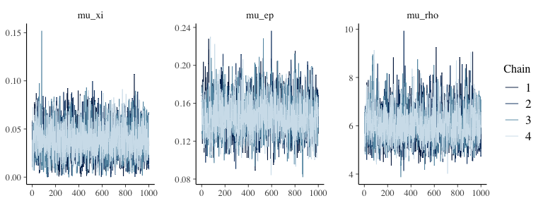

Well-mixed traces look like “fuzzy caterpillars” and confirm what the $\hat{R}$ values suggest (see this StackExchange thread for why mixing matters). Trace plots show post-warmup draws only.

For posterior interval / density plots of the hyper-parameters:

plot(output1, type="simple")  # bayesplot::mcmc_intervals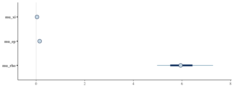

plot(output1)                 # type="dist" — per-model density plots

## Warning: The dot-dot notation (`..density..`) was deprecated in ggplot2 3.4.0.
## ℹ Please use `after_stat(density)` instead.
## ℹ The deprecated feature was likely used in the hBayesDM package.
##   Please report the issue at <https://github.com/CCS-Lab/hBayesDM/issues>.
## This warning is displayed once per session.
## Call `lifecycle::last_lifecycle_warnings()` to see where this warning was
## generated.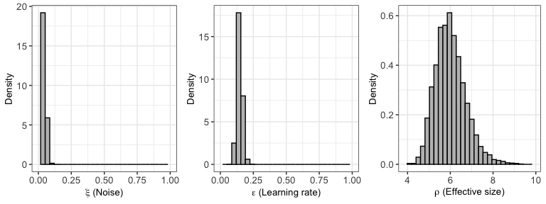

To inspect individual subjects, use plot_ind() (built on bayesplot::mcmc_areas / mcmc_intervals). For example, each subject’s $\epsilon$ (learning rate) posterior:

plot_ind(output1, "ep")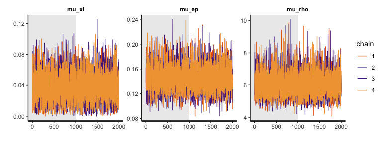

You can also call rhat(output1) to get a data.frame of Rhat values, or rhat(output1, less = 1.05) to get a TRUE/FALSE summary check.

4) Compare models (and groups)

To compare models, you first fit all models in the same manner as the example above (e.g., output4 = gng_m4("example", niter=2000, nwarmup=1000, nchain=4, ncore=4) ). Next, we use the command print_fit, which is a convenient way to summarize Leave-One-Out Information Criterion (LOOIC) or Widely Applicable Information Criterion (WAIC) of all models we consider (see Vehtari et al. (2015) for the details of LOOIC and WAIC). By default, print_fit function uses the LOOIC which is preferable to the WAIC when there are influential observations (Vehtari et al., 2015).

Assuming four models’ outputs are output1 (gng_m1), output2 (gng_m2), output3 (gng_m3), and output4 (gng_m4), their model fits can be simultaneously summarized by:

> print_fit(output1, output2, output3, output4)
   Model    LOOIC
1 gng_m1 1588.843
2 gng_m2 1571.129
3 gng_m3 1573.872
4 gng_m4 1543.335

Note that the lower LOOIC is, the better its model-fit is. Thus, model#4 has the best LOOIC compared to other models. Users can print WAIC or both by calling print_fit(output1, output2, output3, output4, ic="waic") or print_fit(output1, output2, output3, output4, ic="both"). Use the extract_ic function (e.g., extract_ic(output3) ) if you want more detailed information including standard errors and expected log pointwise predictive density (elpd). Note that the extract_ic function can be used only for a single model output.

We also want to remind you that there are multiple ways to compare computational models (e.g., simulation method (absolute model performance), parameter recovery, generalization criterion) and the goodness of fit (e.g., LOOIC or WAIC) is just one of them. Check if predictions from your model (e.g., “posterior predictive check”) can mimic the data (same data or new data) with reasonable accuracy. See Kruschke (2014) (for posterior predictive check), Guitart-Masip et al. (2012) (for goodness of fit and simulation performance on the orthogonalized Go/Nogo task), and Busemeyer & Wang (2000) (for generalization criterion) as well as Ahn et al. (2008; 2014) and Steingroever et al. (2014) (for the combination of multiple model comparison methods).

To compare two groups in a Bayesian fashion (e.g., Ahn et al., 2014), first you need to fit each group with the same model and ideally the same number of MCMC samples. For example,

data_group1 = "~/Project_folder/gng_data_group1.txt"  # data file for group1
data_group2 = "~/Project_folder/gng_data_group2.txt"  # data file for group2

output_group1 = gng_m4(data_group1)  # fit group1 data with the gng_m4 model
output_group2 = gng_m4(data_group2)  # fit group2 data with the gng_m4 model

## After model fitting is complete for both groups,
## evaluate the group difference (e.g., on the 'pi' parameter) by examining the posterior distribution of group mean differences.

diffDist = output_group1$par_vals$mu_pi - output_group2$par_vals$mu_pi  # group1 - group2
hdi( diffDist )  # Compute the 95% Highest Density Interval (HDI).
plot_hdi( diffDist )    # plot the group mean differences

5) Extracting trial-by-trial regressors for model-based fMRI/EEG analysis

In model-based neuroimaging (e.g., O’Doherty et al., 2007), model-based time series of a latent cognitive process are generated by computational models, and then time series data are convolved with a hemodynamic response function and regressed again fMRI or EEG data. This model-based neuroimaging approach has been particularly popular in cognitive neuroscience.

The biggest challenge for performing model-based fMRI/EEG is to learn how to extract trial-by-trial model-based regressors. The hBayesDM package allows users to easily extract model-based regressors that can be used for model-based fMRI or EEG analysis. The hBayesDM package currently provides the following model-based regressors. With the trial-by-trial regressors, users can easily use their favorite neuroimaging package (e.g., in Statistical Parametric Mapping (SPM; http://www.fil.ion.ucl.ac.uk/spm/) to perform model-based fMRI analysis. See our paper (Extracting Trial-by-Trial Regressors for Model-Based fMRI/EEG Analysis) for more details.

As an example, if you would like to extract trial-by-trial stimulus values (i.e., expected value of stimulus on each trial), first fit a model like the following (set the model_regressor input variable to TRUE. Its default value is FALSE):

## fit example data with the gng_m3 model
output3 = gng_m3(data="example", niter=2000, nwarmup=1000, model_regressor=TRUE)

## Warning in gng_m3(data = "example", niter = 2000, nwarmup = 1000, nchain = 4, : Number of cores specified for parallel computing greater than number of locally available cores. Using all locally available cores.

## 
## Model name  = gng_m3 
## Data file   = example 
## 
## Details:
##  # of chains                    = 4 
##  # of cores used                = 3 
##  # of MCMC samples (per chain)  = 2000 
##  # of burn-in samples           = 1000 
##  # of subjects                  = 10 
##  # of (max) trials per subject  = 240 
## 
## **************************************
## **  Extract model-based regressors  **
## **************************************
## 
## 
## ****************************************
## ** Use VB estimates as initial values **
## ****************************************
## ------------------------------------------------------------ 
## EXPERIMENTAL ALGORITHM: 
##   This procedure has not been thoroughly tested and may be unstable 
##   or buggy. The interface is subject to change. 
## ------------------------------------------------------------ 
## Gradient evaluation took 0.000695 seconds 
## 1000 transitions using 10 leapfrog steps per transition would take 6.95 seconds. 
## Adjust your expectations accordingly! 
## Begin eta adaptation. 
## Iteration:   1 / 250 [  0%]  (Adaptation) 
## Iteration:  50 / 250 [ 20%]  (Adaptation) 
## Iteration: 100 / 250 [ 40%]  (Adaptation) 
## Iteration: 150 / 250 [ 60%]  (Adaptation) 
## Iteration: 200 / 250 [ 80%]  (Adaptation) 
## Success! Found best value [eta = 1] earlier than expected. 
## Begin stochastic gradient ascent. 
##   iter             ELBO   delta_ELBO_mean   delta_ELBO_med   notes  
##    100         -829.292             1.000            1.000 
##    200         -817.856             0.507            1.000 
##    300         -818.345             0.338            0.014 
##    400         -816.956             0.254            0.014 
##    500         -816.838             0.203            0.002   MEDIAN ELBO CONVERGED 
## Drawing a sample of size 1000 from the approximate posterior...  
## COMPLETED. 
## Finished in  4.1 seconds.
## 
## ************************************
## **** Model fitting is complete! ****
## ************************************

Once the sampling is completed, all model-based regressors are contained in the model_regressor list.

## store all subjects' stimulus value (SV) in ‘sv_all’
sv_all = output3$model_regressor$SV

dim(output3$model_regressor$SV)  # number of rows=# of subjects (=10), number of columns=# of trials (=240)

## [1]  10 240

## visualize SV (Subject #1)
plot(sv_all[1, ], type="l", xlab="Trial", ylab="Stimulus Value (subject #1)")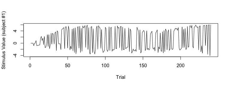

## visualize SV (Subject #5)
plot(sv_all[5, ], type="l", xlab="Trial", ylab="Stimulus Value (subject #5)")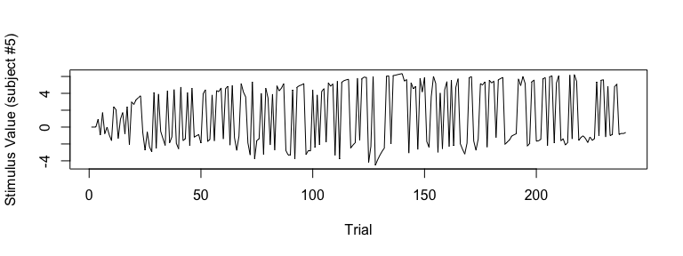

Similarly, users can extract and visualize other model-based regressors. W(Go), W(NoGo), Q(Go), Q(NoGo) are stored in Wgo, Wnogo, Qgo, and Qnogo, respectively.

6) Variational inference for approximate posterior sampling

Set vb = TRUE (default FALSE) to use Stan’s variational algorithm — cmdstanr::CmdStanModel$variational() under the hood — for approximate posterior sampling. VB completes in seconds and is useful for quick exploration, but final inferences should use MCMC.

To run gng_m3 with VB:

output3 = gng_m3(data="example", vb = TRUE)

MCMC arguments (nchain, niter, nthin, nwarmup) don’t apply when vb = TRUE. The returned fit is a CmdStanVB object instead of CmdStanMCMC. See ?cmdstanr::CmdStanModel$variational for the underlying Stan options.

7) Posterior predictive checks

Simply put, posterior predictive checks refer to when a fitted model is used to generate simulated data and check if simulated data are similar to the actual data. Posterior predictive checks are useful in assessing if a model generates valid predictions.

From v0.5.0, users can run posterior predictive checks on all models except drift-diffusion models in hBayesDM. Simulated data from posterior predictive checks are contained in hBayesDM_OUTPUT$par_vals$y_pred. In a future release, we will include a function/command that can conveniently summarize and plot posterior predictive checks. In the mean time, users can program their own codes like the following:

## fit example data with the gng_m3 model and run posterior predictive checks
x = gng_m3(data="example", niter=2000, nwarmup=1000, nchain=4, ncore=4, inc_postpred = TRUE)

## dimension of x$par_vals$y_pred
dim(x$par_vals$y_pred)   # y_pred --> 4000 (MCMC samples) x 10 (subjects) x 240 (trials)
[1] 4000  10  240

y_pred_mean = apply(x$par_vals$y_pred, c(2,3), mean)  # average of 4000 MCMC samples

dim(y_pred_mean)  # y_pred_mean --> 10 (subjects) x 240 (trials)
[1]  10 240

numSubjs = dim(x$all_ind_pars)[1]  # number of subjects

subjList = unique(x$raw_data$subjID)  # list of subject IDs
maxT = max(table(x$raw_data$subjID))  # maximum number of trials
true_y = array(NA, c(numSubjs, maxT)) # true data (`true_y`)

## true data for each subject
for (i in 1:numSubjs) {
  tmpID = subjList[i]
  tmpData = subset(x$raw_data, subjID == tmpID)
  true_y[i, ] = tmpData$keyPressed  # only for data with a 'choice' column
}

## Subject #1
plot(true_y[1, ], type="l", xlab="Trial", ylab="Choice (0 or 1)", yaxt="n")
lines(y_pred_mean[1,], col="red", lty=2)
axis(side=2, at = c(0,1) )
legend("bottomleft", legend=c("True", "PPC"), col=c("black", "red"), lty=1:2)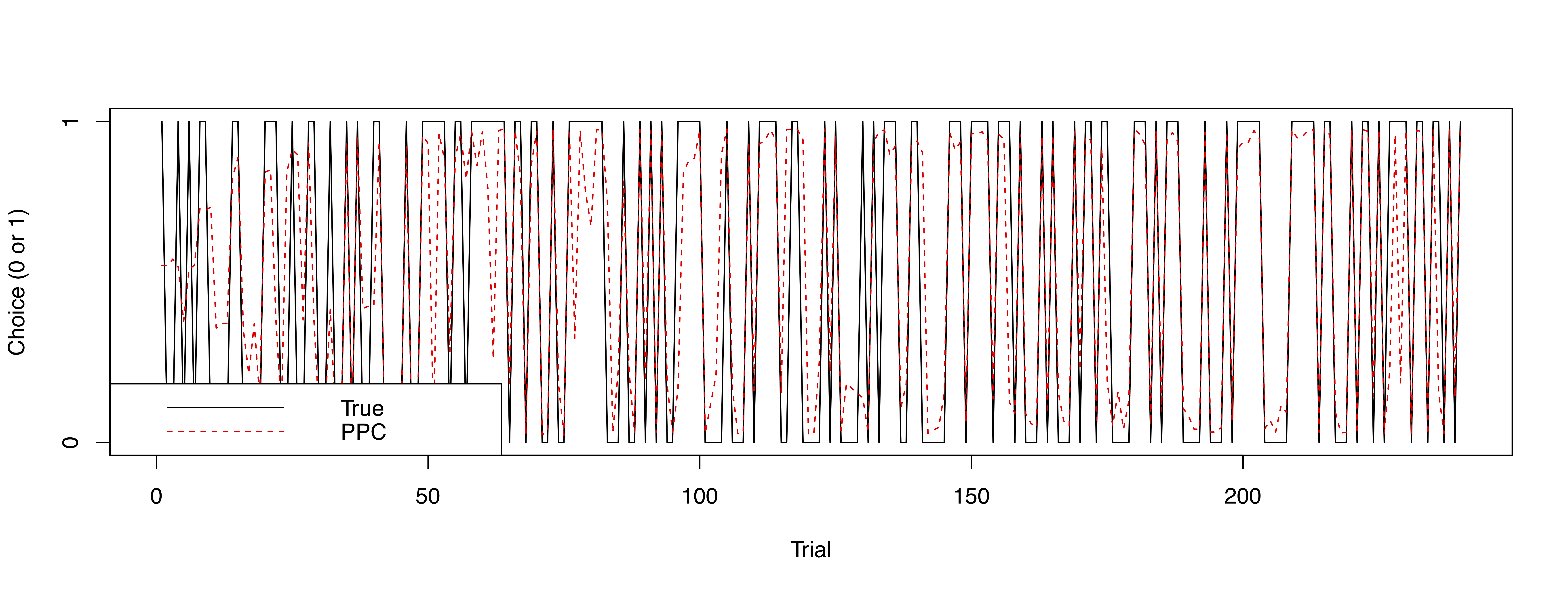

To-do list

We are planning to add more tasks/models. We plan to include the following tasks and/or models in the near future. If you have any requests for a specific task or a model, please let us know.

More sequential sampling models (e.g., drift diffusion models with different drift rates for multiple conditions).
Models for the passive avoidance learning task (Newman et al., 1985; Newman & Kosson, 1986).
Models for the Stop Signal Task (SST)
Allowing users to extract model-based regressors (O’Doherty et al., 2007) from more tasks.

Citation

If you used hBayesDM or some of its codes for your research, please cite this paper:

@article{hBayesDM,
  title = {Revealing Neurocomputational Mechanisms of Reinforcement Learning and Decision-Making With the {hBayesDM} Package},
  author = {Ahn, Woo-Young and Haines, Nathaniel and Zhang, Lei},
  journal = {Computational Psychiatry},
  year = {2017},
  volume = {1},
  pages = {24--57},
  publisher = {MIT Press},
  url = {doi:10.1162/CPSY_a_00002},
}

Papers citing hBayesDM

Here is a selected list of papers that we know that used or cited hBayesDM (from Google Scholar). Let us know if you used hBayesDM for your papers!

Papers citing hBayesDM (Google Scholar)

Acknowledgement

This work was supported in part by the National Institute on Drug Abuse (NIDA) under award number R01DA021421 (PI: Jasmin Vassileva).

References

Ahn, W.-Y., Krawitz, A., Kim, W., Busemeyer, J. R., & Brown, J. W. (2011). A model-based fMRI analysis with hierarchical bayesian parameter estimation. Journal of Neuroscience, Psychology, and Economics, 4(2), 95.

Ahn, W.-Y., Vasilev, G., Lee, S.-H., Busemeyer, J. R., Kruschke, J. K., Bechara, A., & Vassileva, J. (2014). Decision-making in stimulant and opiate addicts in protracted abstinence: Evidence from computational modeling with pure users. Frontiers in Psychology, 5, 849.

Busemeyer, J. R., & Diederich, A. (2010). Cognitive modeling. Sage Publications, Inc.

Busemeyer, J. R., & Wang, Y.-M. (2000). Model comparisons and model selections based on generalization criterion methodology. Journal of Mathematical Psychology, 44, 171–189.

Daw, N. D. (2011). Trial-by-trial data analysis using computational models. Decision Making, Affect, and Learning: Attention and Performance XXIII, 23, 3–38.

Huys, Q. J. M., Cools, R., Gölzer, M., Friedel, E., Heinz, A., Dolan, R. J., & Dayan, P. (2011). Disentangling the roles of approach, activation and valence in instrumental and pavlovian responding. PLoS Computational Biology, 7(4), e1002028.

Kruschke, J. (2014). Doing bayesian data analysis: A tutorial with R, JAGS, and Stan. Academic Press.

Lee, M. D. (2011). How cognitive modeling can benefit from hierarchical bayesian models. Journal of Mathematical Psychology, 55(1), 1–7.

Lee, M. D., & Wagenmakers, E.-J. (2014). Bayesian cognitive modeling: A practical course. Cambridge University Press.

Newman, J. P., & Kosson, D. S. (1986). Passive avoidance learning in psychopathic and nonpsychopathic offenders. Journal of Abnormal Psychology, 95(3), 252.

Newman, J. P., Widom, C. S., & Nathan, S. (1985). Passive avoidance in syndromes of disinhibition, psychopathy, and extraversion. Journal of Personality and Individual Differences, 48, 1316–1327.

O’Doherty, J. P., Hampton, A., & Kim, H. (2007). Model-based fMRI and its application to reward learning and decision making. Annals of the New York Academy of Sciences, 1104(1), 35–53.

Shiffrin, R. M., Lee, M. D., Kim, W., & Wagenmakers, E. J. (2008). A survey of model evaluation approaches with a tutorial on hierarchical Bayesian methods. Cognitive Science: A Multidisciplinary Journal, 32(8), 1248–1284.

Steingroever, H., Wetzels, R., & Wagenmakers, E.-J. (2014). Absolute performance of reinforcement-learning models for the iowa gambling task. Decision, 1(3), 161.

Vehtari, A., Gelman, A., & Gabry, J. (2015). Efficient implementation of leave-one-out cross-validation and WAIC for evaluating fitted Bayesian models. arXiv Preprint arXiv:1507.04544.