Hierarchical Bayesian Analysis on Hierarchical Gaussian Filter
Source:vignettes/hgf_tutorial.Rmd
hgf_tutorial.RmdBy Jinwoo Jeong, Juha Lee, Yusom Jo, Woo-Young Ahn | September 2, 2025
Hierarchical Gaussian Filter (HGF) is a computational model designed to explain how individuals learn in uncertain and changing environments (Mathys et al., 2011). Currently, TAPAS is the most widely used tool for applying HGF to behavioral data. By offering various combinations of perceptual and observation models, TAPAS HGF Toolbox enabled a computationally efficient way to apply different HGF models (also see PyHGF, a Python-library, which supports generalized HGF models).
Here, we show how we implemented HGF in the hBayesDM
1.3.0 (Ahn et al., 2017). Two
new HGF models are included in the package: hgf_ibrb (for
hierarchical Bayesian analysis) and hgf_ibrb_single
(for individual Bayesian analysis). ibrb refers to input =
binary & response = binary. Although these functions are currently
limited to behavioral data with binary inputs and binary responses, they
provide a straightforward way to apply MCMC and (hierarchical) Bayesian
analysis to HGF models, which are currently unavailable in TAPAS.
1. Example Task
Let’s consider a probabilistic reversal learning task where HGF can be applied.
On each trial, participants are presented with two colored options—blue(1) and orange(0)—and choose one of the options. Reward contingency changes over trials (see Figure 1) and participants are instructed to maximize the cumulative reward.
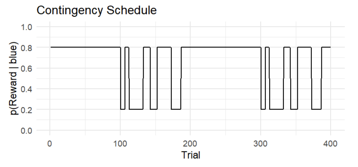
Figure 1. Reward contingency schedule. The y-axis shows the actual reward probability of the blue option p(reward|blue), while the x-axis shows the trial number. Note that p(reward|orange) = 1 - p(reward|blue).
The figure above illustrates a contingency schedule for a restless two-armed bandit task. The schedule spans 400 trials, alternating between stable and volatile phases.
- Stable phases (100 trials each): reward probabilities remain fixed. For example, choosing the blue option yields a reward with a probability of 80% throughout the first stable block.
- Volatile phases (100 trials each): reward probabilities switch between 20% and 80% after a random number of trials (6, 10, 14, or 20), making the environment unpredictable.
Probabilistic learning tasks like this are well suited for HGF analysis because the environment changes over time, requiring participants to continuously track shifting reward contingencies.
2. Understanding HGF
In this section, we briefly explain HGF (please see Mathys et al., 2011, 2014 for more details). One way to approach probabilistic learning tasks is to assume a “true” hidden quantity for each trial, such as the actual probability of receiving a reward from the chosen option. This hidden state changes over time according to the contingency schedule, but the agent cannot observe it directly. Instead, the agent tries to update its beliefs about the hidden state across trials based on inputs and observed feedback (whether the chosen option led to a reward or not). In this sense, the task represents a learning problem under uncertainty: how an agent can keep track of a changing, probabilistic world based on noisy feedback.
Note that there exist multiple sources of uncertainty: stochasticity (the reward is probabilistic on each trial), volatility (the reward contingency changes over time), and even volatility of volatility (the degree of environmental change itself may vary over time). Successful performance on such a task therefore depends on the optimal processing of these sources of uncertainty in learning, and the pattern of such processing can be characterized by the parameter values in HGF.
2.1. Model Structure
As the name suggests, the Hierarchical Gaussian Filter consists of multiple levels of hidden states, each of which are organized in a hierarchy and evolving in Gaussian random walks. Theoretically, the number of hierarchy levels has no upper bound, but in practice it is not set too high due to diminishing explanatory gains and limited interpretability as a cognitive model.
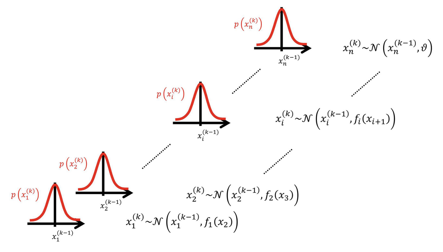
Figure 2. Overview of the Hierarchical Gaussian Filter (adopted from Mathys et al. 2014)
For instance, let’s assume a 3-level HGF with binary inputs and binary responses. An HGF model with 3 levels has three (hidden) states for each level: x₁, x₂, x₃. And each state represents a different aspect of the environment.
Level 1 (x₁) is the lowest level, representing the immediate observation or perceptual state. For example, in a binary task, x₁ might be the state of a cue or outcome coded as 0 or 1. This level does not evolve via a random walk, instead, it is generated from x₂ through an observation model (e.g., Bernoulli for binary outcomes). When there is no sensory noise, x₁ directly corresponds to the observed input.
Level 2 (x₂) is a hidden state that represents the current contingency of the environment (e.g., the probability of a binary outcome). It can be thought of as the agent’s belief about the latent factor governing level-1 events. This is a continuous state that drifts over time via a Gaussian random walk: on each trial, x₂ changes slightly, with the variance of this change dictated by level 3 (x₃).
Level 3 (x₃) is a higher-level hidden state representing the volatility of the environment, namely how rapidly x₂ changes. Although x₃ is modeled as a Gaussian random walk, the variance of this random walk is determined by a constant parameter because there is no higher level to modulate it. Intuitively, when x₃ is high, the agent believes the environment is changing rapidly and therefore updates x₂ more strongly; when x₃ is low, the agent assumes stability and updates x₂ more conservatively.
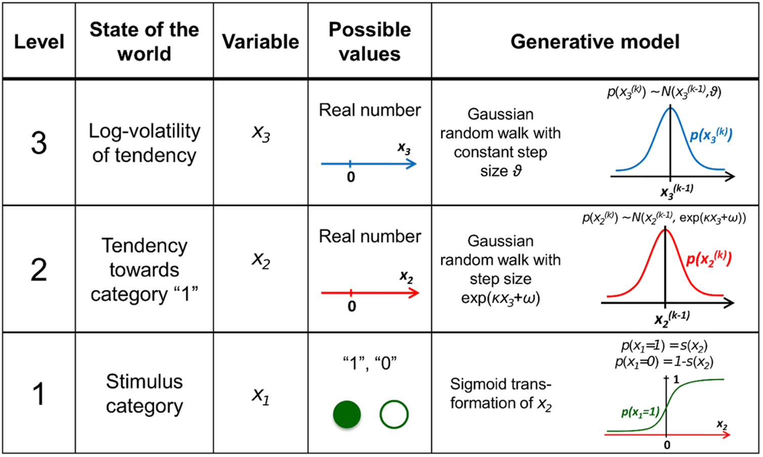
Figure 3. Overview of the hierarchical generative model (Mathys et al. 2011)
2.2. Perceptual model
In the HGF perceptual model, the parameters κ (kappa) and ω (omega) regulate the coupling and dynamics across hierarchical levels. They encode the agent’s prior assumptions about environmental uncertainty and determine how learning adapts to changing conditions.
At each level \(l\), the state \(x_l\) at trial \(k\) evolves as a Gaussian random walk whose variance depends on κ and ω:
\[\begin{align*} x_l^{(k)} &\sim N\bigl(x_l^{(k-1)} \text{, } \exp(\kappa_l x_{l+1}^{(k)} + \omega_l )\bigr), \quad l=2,...L-1 \\ \end{align*}\]
At the top level \(L\), the variance depends only on ω:
\[\begin{align*} x_L^{(k)} &\sim N\bigl(x_L^{(k-1)} \text{, } \exp(\omega_L )\bigr) \end{align*}\]
κ: phasic volatility
κ determines how strongly a lower-level state is influenced by the state above it. Formally, it scales the effect of the higher-level value on the variance of the lower-level random walk. In a perception model with binary inputs and \(L\) hierarchical levels, κ is defined for levels 2 through \(L-1\).
κ must be non-negative, and it has been suggested that an upper bound at or below 2 is sensible (Mathys et al., 2014).
- When κ is too small, the lower level is almost decoupled from the higher one. Even if the higher-level state signals increased volatility, the learning rate at the lower level hardly changes. The agent ends up learning at a nearly fixed pace regardless of environmental instability.
- When κ is too large, even small changes in the higher-level state strongly alter the lower-level learning rate. For instance, if volatility spikes, the agent immediately increases its learning rate. This makes the agent very adaptive, but it can also lead to overreacting to random noise.
ω: tonic volatility
ω provides the baseline drift for each level’s random walk. It is the constant offset in the log-variance, setting how much the agent expects change even without higher-level modulation. In a perception model with binary inputs and \(L\) hierarchical levels, ω is defined for levels 2 through \(L\).
Theoretically, ω doesn’t require upper or lower bounds. However, both
hgf_ibrb and hgf_ibrb_single
require setting the appropriate range for each level of ω parameters for
efficient and effective sampling.
- When ω is too low, the random walk variance is small by default. The agent assumes stability, so updates are slow and conservative. Even with repeated prediction errors, beliefs change only gradually, reflecting a tendency to cling to prior expectations.
- When ω is too high, the random walk variance is very large by default. The agent assumes that environmental changes are common, so it updates beliefs quickly, even in a stable environment. This can capture individuals’ characteristics who are highly responsive or prone to “jumping to conclusions.”
2.3. Response model
The response model maps the agent’s internal prediction onto an
observable decision. In both hgf_ibrb and hgf_ibrb_single,
the unit-square sigmoid function is used to transform a predictive
probability 𝑚∈[0,1] into a binary choice probability:
\[ p(y = 1) = \frac{m^{\text{ }\zeta}}{m^{\text{ }\zeta} + (1 - m)^{\zeta}} \]
ζ: inverse decision noise
The parameter ζ (zeta) controls the steepness of the unit-square sigmoid, regulating the stochasticity of decision-making. ζ is defined only for level 1 and must be non-negative.
- When ζ is low, the sigmoid curve becomes shallow. Even strong predictions (e.g., 𝑚 = 0.8) yield only moderate choice biases, and choices remain noisy and weakly belief-driven.
- When ζ is high, the sigmoid curve becomes steep. Even very small deviations from 0.5 lead to near-deterministic choices, and behavior closely follows the agent’s beliefs.
3. Tutorial on hgf_ibrb and
hgf_ibrb_single
This section explains how we can actually run hgf_ibrb and hgf_ibrb_single.
The examples are based on the R version of the hBayesDM
package, but both functions are also implemented in the Python version
of the hBayesDM package.
3.1. Setup
hBayesDM setup
Check the Getting Started page
to set up hBayesDM.
Prepare your data
For simple tests, hBayesDM has example data for both hgf_ibrb and hgf_ibrb_single.
If you want to apply HGF on your own data, make sure that your file
has the .csv or .tsv format and contains these
four columns.
-
subjID: unique subject identifier (integer or string) -
trialNum: trial index (1, 2, 3, …) -
u: input on that trial (0 or 1) -
y: subject’s choice on that trial (0 or 1)
For example, the task design in Section 1
provides two colored options: blue coded as 1 and orange coded as 0. In
this case, a participant (subjID = 1) can choose the blue
option (y = 1) at the first trial
(trialNum = 1) when the correct choice was actually the
orange option (u = 0). No other information (e.g.,
feedback column indicating whether the subject got the
reward or not) is needed in the HGF model.
3.2. Fitting with default settings
Now, we will share various ways we can fit hgf_ibrb and hgf_ibrb_single
on the example data.
Below is the simplest way to run hgf_ibrb on a dataset
with multiple participants. The command below initiates an MCMC
procedure of 4 MCMC chains, each consisting of 500 burn-in (warm-up)
iterations followed by 500 sampling iterations.
fit <- hgf_ibrb(data = "example", niter = 1000, nwarmup = 500, nchain = 4)The above command is the same as the commands below because
unspecified arguments fall back to their default values. By default, hgf_ibrb fits a
3-level HGF model (L = 3). The kappa_lower and
kappa_upper arguments are one-element vectors that bound
κ₂, whereas omega_lower and omega_upper are
two-element vectors that bound ω₂ and ω₃. In contrast,
zeta_lower and zeta_upper are scalars, since
there is only a single ζ regardless of the hierarchy depth.
fit <- hgf_ibrb(
  data = "example",
  niter = 1000,
  nwarmup = 500,
  nchain = 4,
  L = 3,
  input_first = FALSE,
  mu0 = c(0.5, 1.0),
  sigma0 = c(0.1, 1.0),
  kappa_lower = c(0),
  kappa_upper = c(2),
  omega_lower = c(-10, -15),
  omega_upper = c(0, 0),
  zeta_lower  = 0,
  zeta_upper  = 2
)
Below are some of the simple ways to print the overall statistics of the fitted results.
To apply HGF to a single participant’s data, you can use hgf_ibrb_single
like below.
fit <- hgf_ibrb_single(data = "example", niter = 1000, nwarmup = 500, nchain = 4)
print(summary(fit))
print(fit$all_ind_pars)3.3. input_first option
The input_first option is to help researchers apply HGF
without changing their data format.
- input_first=TRUE: for each row, participant observed the value of
input
ubefore choosingy - input_first=FALSE: for each row, participant observed the value of
input
uafter choosingy(default)
fit <- hgf_ibrb(data = "example", niter = 1000, nwarmup = 500, nchain = 4, input_first=TRUE)Similar features are also implemented in the observation models in
TAPAS as the predorpost configuration.
3.4. Parameter boundaries
Parameter boundaries can be set for each parameter. For example, if you want to set parameter boundaries for a 3-level HGF model as:
\[\begin{align*} 0 < &\text{ }\kappa < 1 \\ -10 < &\text{ }\omega_{2} < 2 \\ -15 < &\text{ }\omega_{3} < 3 \\ 0 < &\text{ }\zeta < 4 \end{align*}\]
Then, you set the arguments below:
3.5. Fixing parameter values
As TAPAS provides a way to fixate a certain parameter to a fixed
value, hgf_ibrb
and hgf_ibrb_single
also provide a similar feature. To set a parameter as a constant, simply
set the lower bound and upper bound to the same value. Below are some
examples.
The command below fixates κ value to 1, while other parameters are set as free parameters with their default boundaries.
The command below fixates ω₂ to -4, while ω₃ is still estimated with the given boundaries (-10 < ω₃ < -2).
In contrast, the command below fixates ω₃ to -4, while ω₂ is still to be estimated with the given boundaries (-9 < ω₂ < -1).
The command below fixates ζ value to 1, while other parameters are estimated with default boundaries.
fit <- hgf_ibrb(data = "example", zeta_lower = 1.0, zeta_upper = 1.0)Of course, you can fixate multiple parameters at the same time as shown below:
3.6. L: level of hierarchy
L option can be used to specify the level of hierarchy.
The default and the minimum value is L=3 because it is the
most widely used and most interpretable.
Note that the number of parameters is automatically chosen based on
the level of hierarchy. For example, the code below will fail because
the default arguments for each parameter can only be used for
L = 3.
fit <- hgf_ibrb(data = "example", niter = 1000, nwarmup = 500, nchain = 4, L = 4)Below is an example of fitting a 4-level HGF model. L=4
introduces a fourth latent state (x₄) and extends the parameterization
with two couplings (κ₂, κ₃), volatilities (ω₂, ω₃, ω₄), and
initial-state vectors for levels 2-4.
4. Parameter Recovery
In order to ensure that the estimated parameters genuinely reflect the underlying generative process, parameter recovery analysis was conducted to validate parameter identifiability and estimation reliability. This procedure involves generating synthetic datasets from known parameter values and then re-estimating those parameters using the same model (Ahn et al., 2011; Heathcote et al., 2015; Wilson & Collins, 2019).
4.1. Simulation
In order to simulate binary inputs, the contingency schedule from Section 1 was used to create 400 trials of
inputs. To simulate binary responses, tapas_simModel
function from TAPAS HGF Toolbox was applied to the simulated inputs,
assuming 3-level HGF with binary responses. A total of 30 participants’
behavioral datasets were generated using randomly chosen parameter
combinations:
\[\begin{align*} \kappa &= 1.0 \\ -9.0 \leq &\text{ }\omega_{2} \leq -1.0 \\ -10.0 \leq &\text{ }\omega_{3} \leq -2.0 \\ 0.03 \leq &\text{ }\zeta \leq 4.0 \end{align*}\]
Note that κ is fixed to 1, following many of the previous works with similar context (Hein et al., 2021; Tecilla et al., 2023).
4.2. Recovery with TAPAS
In order to check whether the simulated data had reasonable parameter
ranges that HGF models can recover, tapas_fitModel function
from TAPAS HGF Toolbox was applied to check parameter recovery.
tapas_hgf_binary and tapas_unitsq_sgm models
were applied using the following prior settings:
\[\begin{align*} \mu_{0,2} &= 0, \quad \mu_{0,3} = 1 \\ \sigma^{2}_{0,2} &= 1, \quad \sigma^{2}_{0,3} = 1 \\ \omega_{2} &\sim N(-5, 4^2) \\ \omega_{3} &\sim N(-6, 4^2) \end{align*}\]
Figure 4 shows that both ω₂ and ζ were recovered extremely well (ω₂: r = 0.99, p < 1.63e-23; ζ: r = 0.99, p < 8.9e-26), indicating that these parameters can be reliably estimated at the individual level. In contrast, ω₃ exhibited exhibited poor parameter recovery (r = -0.09, p = 0.633), with all the estimated values presumably stuck in a local minima near -6.
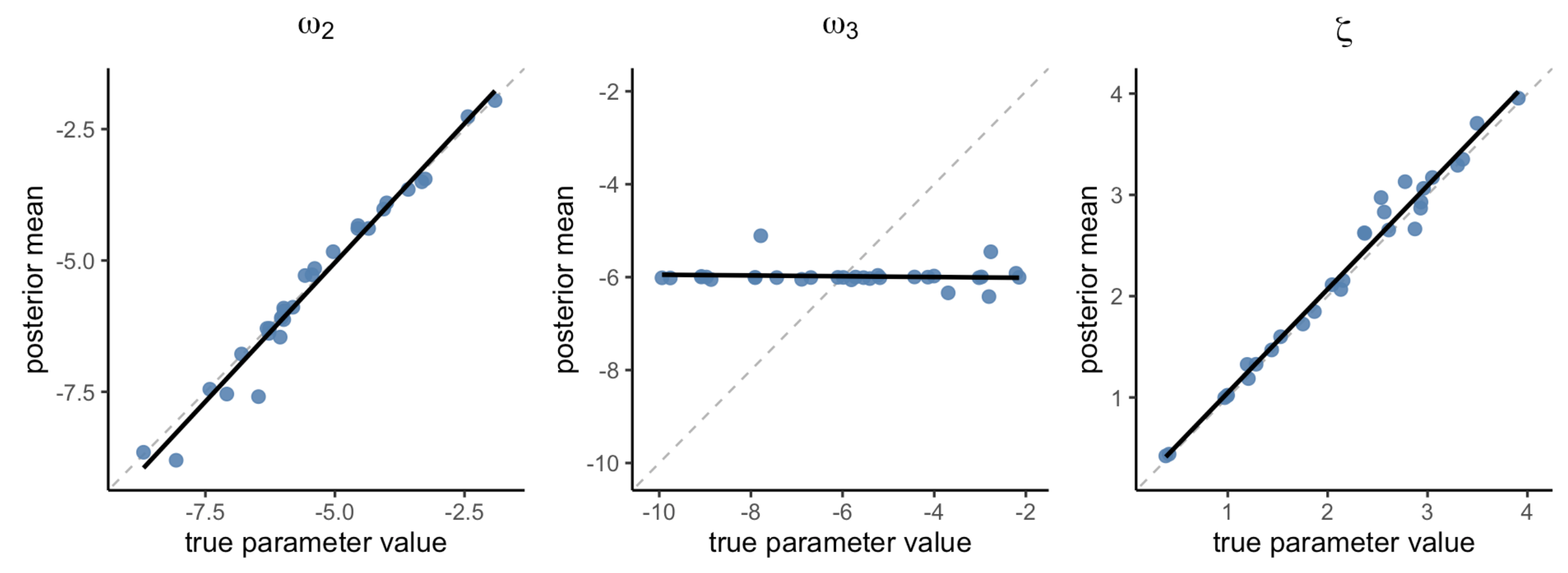
Figure 4. Parameter recovery with TAPAS. Posterior means of the estimated parameters.
4.3. Recovery with hgf_ibrb_single
For each subject’s data, hgf_ibrb_single
was applied in a loop with settings like below.
fit <- hgf_ibrb_single(data = subject_data,
                       niter = 3000,
                       nwarmup = 1500,
                       nchain = 4,
                       L = 3,
                       kappa_lower = c(1.0),
                       kappa_upper = c(1.0),
                       omega_lower = c(-9.0, -10.0),
                       omega_upper = c(-1.0, -2.0),
                       zeta_lower  = 0.03,
                       zeta_upper  = 4.0,
                       mu0 = c(0.0, 1.0),
                       inits = "random"
)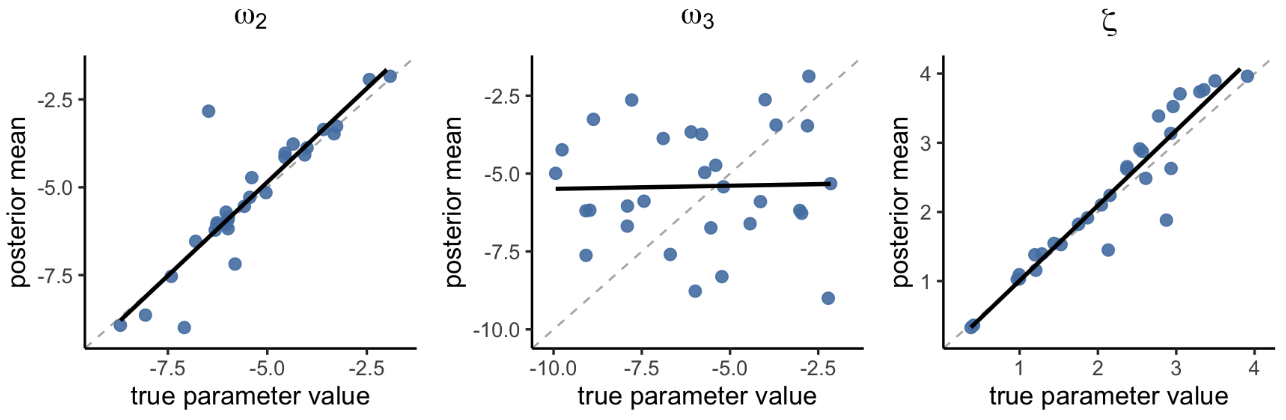
Figure 5. Parameter recovery with hBayesDM (hgf_ibrb_single, individual Bayesian analysis)
Figure 5 shows that both ω₂ and ζ were recovered pretty well (ω₂: r = 0.90, p < 2.51e-11; ζ: r = 0.95, p < 7.81e-16). In contrast, ω₃ showed poor parameter recovery (r = 0.03, p = 0.892).
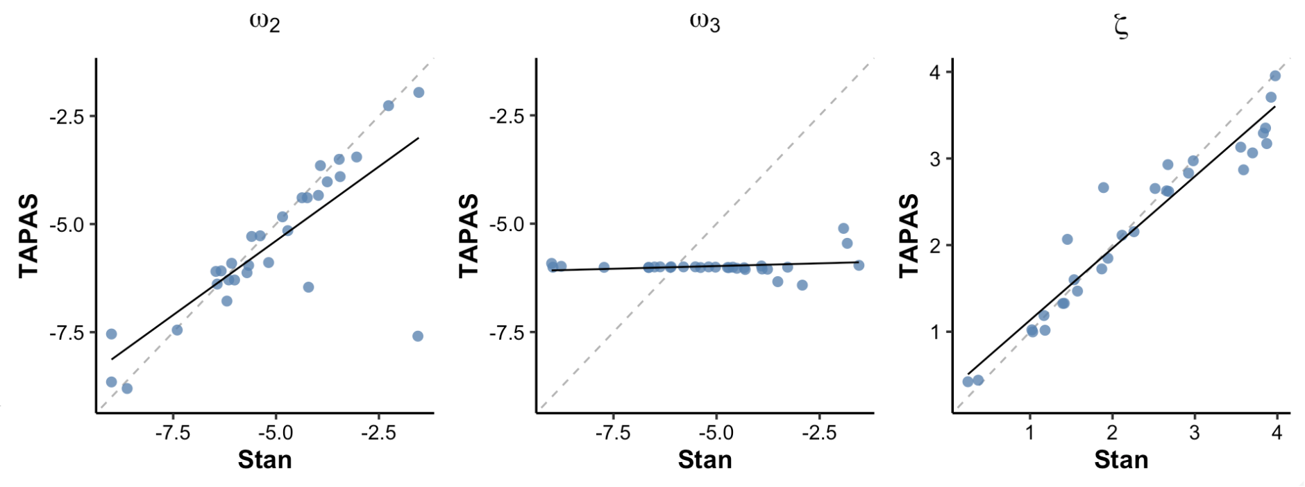
Figure 6. TAPAS vs hgf_ibrb_single
In Figure 6, we compared TAPAS and hBayesDM
(individual-level) parameter estimates. The figure shows that ω₂ and ζ
parameter estimates of hBayesDM and TAPAS are highly
correlated with each other. In contrast, ω₃ estimates are not, but the
comparison may be meaningless considering that both approches failed to
show good parameter recovery of ω₃.
Overall, these results suggest that we can use hBayesDM
for individual level analysis, which yields similar parameter estimates
from using TAPAS. At the same time, hBayesDM yields
posterior distributions instead of points estimates, which provide
additional information about the parameters.
4.4. Recovery with hgf_ibrb
For hierarchical Bayesian analysis, we applied hgf_ibrb to the data
from 30 participants like below:
output <- hgf_ibrb(
  data = data,
  niter = 3000,
  nwarmup = 1500,
  nchain = 4,
  L = 3,
  kappa_lower = c(1.0),
  kappa_upper = c(1.0),
  omega_lower = c(-9.0, -10.0),
  omega_upper = c(-1.0, -2.0),
  zeta_lower  = 0.03,
  zeta_upper  = 4.0,
  mu0   = c(0.0, 1.0),
  inits = "random"
)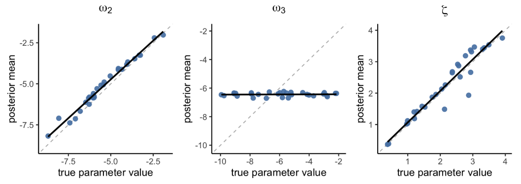
Figure 7. Parameter recovery with hBayesDM (hgf_ibrb, hierarchical Bayesian analysis)
Figure 7 shows that both ω₂ and ζ showed excellent parameter recovery
(ω₂: r = 0.99, p < 1.27e-26; ζ: r = 0.95, p < 2.62e-16), with
better correlation compared to hgf_ibrb_single.
Unfortunately, ω₃ still showed poor recovery (r = 0.06, p = 0.767), but
was slightly better than TAPAS considering that the results from TAPAS
had a negative correlation.
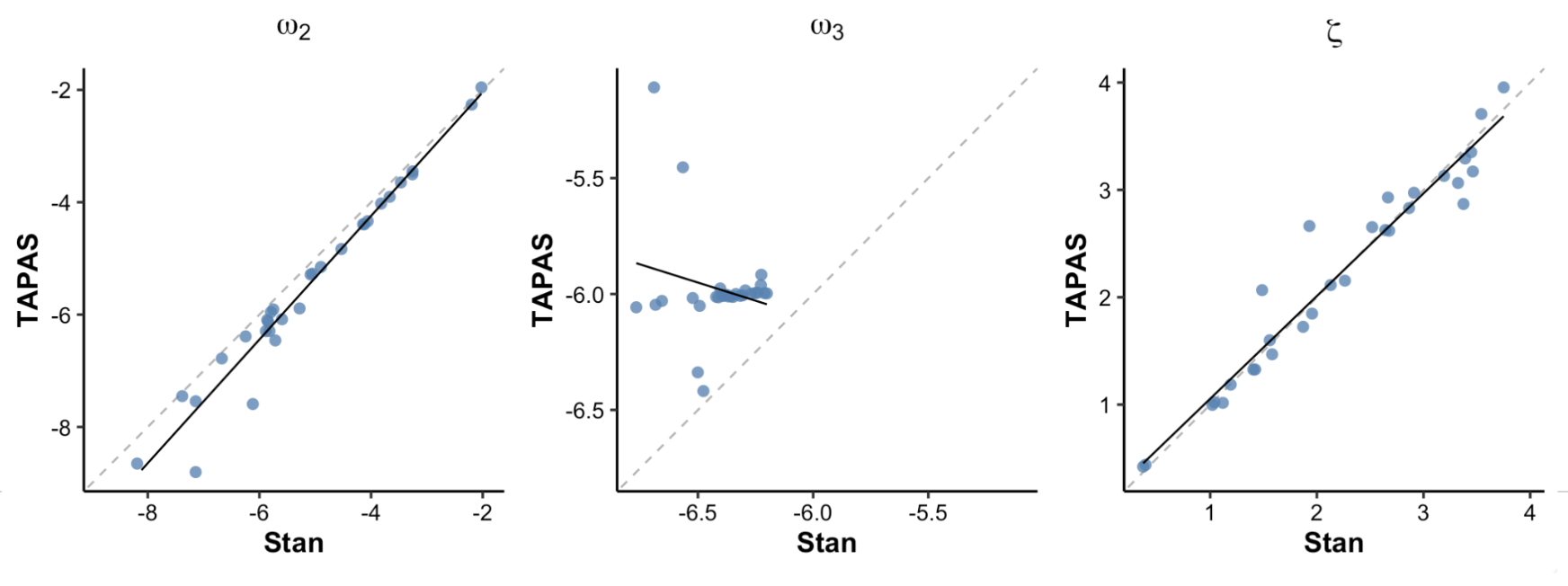
Figure 8. TAPAS vs hgf_ibrb
In Figure 8, we compared TAPAS and hBayesDM (hierarchical Bayesian) parameter estimates. Figure 8 shows that ω₂ and ζ parameter estimates of hBayesDM and TAPAS are highly correlated with each other. Once again, ω₃ estimates of the two appraoches are not correlated with each other.
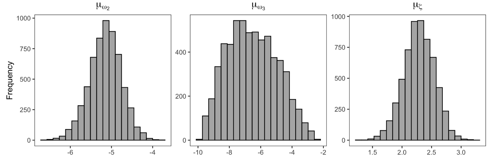
Figure 9. Parameter recovery
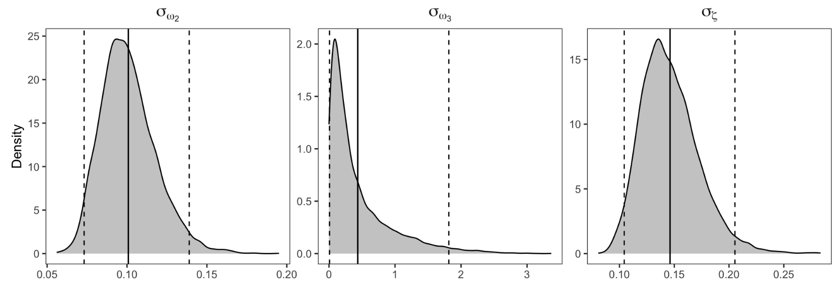
Figure 9. Parameter recovery
Figure 9 shows the posterior distributions for group-level parameters (group means and SDs) for ω₂, ω₃, and ζ, which is an advantage of using MCMC for parameter estimation.
Overall, we conclude hBayesDM provides a user-friendly way of fitting
HGF models whose parameter estimates will be compatible with those from
TAPAS. In many cases, hgf_ibrb should be
preferred over hgf_ibrb_single
as hierarchical modeling framework further improves parameter recovery
compared to individual-level fits, presumably due to the benefits of
shrinkage (Ahn et al., 2011; Kruschke,
2014).
5. Appendix
5.1. Specifying initial values
hBayesDM provides various options for setting the
initial values (inits) of the parameters. The default
setting is vb, therefore hBayesDM will try to
fit the model with variational
inference and then use the VB estimates as initial values for MCMC
sampling. If this VB estimation fails, hBayesDM defaults to
using random initial values instead.
Since the vb option has the issue of failing
stochastically, consider using the random option or
specifying the initial parameter values, like other models implemented
in hBayesDM.
fit <- hgf_ibrb(data = "example", inits = "random")5.2. Poor recovery of ω₃
In Section 4, we showed that both TAPAS and hBayesDM have failed to recover ω₃ properly. In fact, several previous studies have also reported unreliable parameter estimation for ω₃ (Hein et al., 2021; Reed et al., 2020; Tecilla et al., 2023). To our knowledge, there has been no systematic analysis of the causes or the potential solutions. Therefore, we tried various input designs and parameter settings to investigate under what conditions we can achieve decent parameter recovery and ω₃ can produce detectable behavioral differences.
The main issue with the data used in Section 4 was that the individual differences in ω₃ didn’t produce any meaningful differences in the responses between the participants. Thus, we conducted parameter recovery analyses multiple times using various input designs and different ranges of ω₃ (-6.4 < ω₃ < -0.8) while fixing all other parameters. Most promising results were found when we simply added more volatility to the environment using the contingency schedule shown in Figure 10.
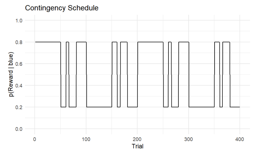
Figure 10. Volatile Contingency Schedule
The overall task design is similar to the Contingency Schedule reported in Section 1. The total number of trials is 400 and switches between stable and volatile phases. The main difference is that number of trials for each stable and volatile phase is 50 trials each, half the number of trials used in the previous design. This leads to twice the number of shifts between stable and volatile phases compared to the previous design.
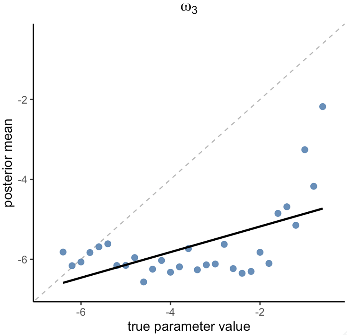
Figure 11. Parameter recovery
Figure 11 shows the result of parameter recovery of ω₃ using hgf_ibrb_single.
Although the results are not perfect, we can see that the parameter
recovery results have improved compared to the results from the previous
design (Figure 5). This indicates that adding enough volatility to the
environment itself is a necessary step for capturing the individual
differences in parameters at high levels such as ω₃.
5.3. Estimating parameters at high levels
Many studies have reported issues in estimating parameters at level 3 or above such as ω₃ (Hein et al., 2021; Reed et al., 2020; Tecilla et al., 2023). Below are some tips to mitigate such issues.
Task design: As mentioned in the previous section, the researcher must carefully design their experiment and check whether their task can appropriately capture the individual differences in the parameters of interest. Simulating experiment data and running parameter recovery before actually conducting the experiment would be the best way to check the task design.
Parameter Boundaries: Setting appropriate parameter boundaries is a crucial part of applying HGF. For instance, if ω₃ is too low, then exp(ω₃) becomes very small (e.g., ω₃ = -8, exp(ω₃) ≈ 0.000335), which means that level-3 updating has almost no influence on the agent’s behavior.